Variational Autoencoder
- Introduction
- VAE: Formulation and Intuition
- VAE: Dissecting the Objective
- Implementation in Keras
- Implementation on MNIST Data
Introduction
There are two generative models facing neck to neck in the data generation business right now: Generative Adversarial Nets (GAN) and Variational Autoencoder (VAE). These two models have different take on how the models are trained. GAN is rooted in game theory, its objective is to find the Nash Equilibrium between discriminator net and generator net. On the other hand, VAE is rooted in bayesian inference, i.e. it wants to model the underlying probability distribution of data so that it could sample new data from that distribution.
VAE: Formulation and Intuition
Suppose we want to generate a data. Good way to do it is first to decide what kind of data we want to generate, then actually generate the data. For example, say, we want to generate an animal. First, we imagine the animal: it must have four legs, and it must be able to swim. Having those criteria, we could then actually generate the animal by sampling from the animal kingdom. Lo and behold, we get Platypus!
From the story above, our imagination is analogous to latent variable. It is often useful to decide the latent variable first in generative models, as latent variable could describe our data. Without latent variable, it is as if we just generate data blindly. And this is the difference between GAN and VAE: VAE uses latent variable, hence it’s an expressive model.
Alright, that fable is great and all, but how do we model that? Well, let’s talk about probability distribution.
Let’s define some notions:
- \( X \): data that we want to model a.k.a the animal
- \( z \): latent variable a.k.a our imagination
- \( P(X) \): probability distribution of the data, i.e. that animal kingdom
- \( P(z) \): probability distribution of latent variable, i.e. our brain, the source of our imagination
- \( P(X \vert z) \): distribution of generating data given latent variable, e.g. turning imagination into real animal
Our objective here is to model the data, hence we want to find \( P(X) \). Using the law of probability, we could find it in relation with \( z \) as follows:
\[ P(X) = \int P(X \vert z) P(z) dz \]
that is, we marginalize out \( z \) from the joint probability distribution \( P(X, z) \).
Now if only we know \( P(X, z) \), or equivalently, \( P(X \vert z) \) and \( P(z) \)…
The idea of VAE is to infer \( P(z) \) using \( P(z \vert X) \). This is make a lot of sense if we think about it: we want to make our latent variable likely under our data. Talking in term of our fable example, we want to limit our imagination only on animal kingdom domain, so we shouldn’t imagine about things like root, leaf, tyre, glass, GPU, refrigerator, doormat, … as it’s unlikely that those things have anything to do with things that come from the animal kingdom. Right?
But the problem is, we have to infer that distribution \( P(z \vert X) \), as we don’t know it yet. In VAE, as it name suggests, we infer \( P(z \vert X) \) using a method called Variational Inference (VI). VI is one of the popular choice of method in bayesian inference, the other one being MCMC method. The main idea of VI is to pose the inference by approach it as an optimization problem. How? By modeling the true distribution \( P(z \vert X) \) using simpler distribution that is easy to evaluate, e.g. Gaussian, and minimize the difference between those two distribution using KL divergence metric, which tells us how difference it is \(P\) and \(Q\).
Alright, now let’s say we want to infer \( P(z \vert X) \) using \( Q(z \vert X) \). The KL divergence then formulated as follows:
Recall the notations above, there are two things that we haven’t use, namely \( P(X) \), \( P(X \vert z) \), and \( P(z) \). But, with Bayes’ rule, we could make it appear in the equation:
Notice that the expectation is over \( z \) and \( P(X) \) doesn’t depend on \( z \), so we could move it outside of the expectation.
If we look carefully at the right hand side of the equation, we would notice that it could be rewritten as another KL divergence. So let’s do that by first rearranging the sign.
And this is it, the VAE objective function:
At this point, what do we have? Let’s enumerate:
- \( Q(z \vert X) \) that project our data \( X \) into latent variable space
- \( z \), the latent variable
- \( P(X \vert z) \) that generate data given latent variable
We might feel familiar with this kind of structure. And guess what, it’s the same structure as seen in Autoencoder! That is, \( Q(z \vert X) \) is the encoder net, \( z \) is the encoded representation, and \( P(X \vert z) \) is the decoder net! Well, well, no wonder the name of this model is Variational Autoencoder!
VAE: Dissecting the Objective
It turns out, VAE objective function has a very nice interpretation. That is, we want to model our data, which described by \( \log P(X) \), under some error \( D_{KL}[Q(z \vert X) \Vert P(z \vert X)] \). In other words, VAE tries to find the lower bound of \( \log P(X) \), which in practice is good enough as trying to find the exact distribution is often untractable.
That model then could be found by maximazing over some mapping from latent variable to data \( \log P(X \vert z) \) and minimizing the difference between our simple distribution \( Q(z \vert X) \) and the true latent distribution \( P(z) \).
As we might already know, maximizing \( E[\log P(X \vert z)] \) is a maximum likelihood estimation. We basically see it all the time in discriminative supervised model, for example Logistic Regression, SVM, or Linear Regression. In the other words, given an input \( z \) and an output \( X \), we want to maximize the conditional distribution \( P(X \vert z) \) under some model parameters. So we could implement it by using any classifier with input \( z \) and output \( X \), then optimize the objective function by using for example log loss or regression loss.
What about \( D_{KL}[Q(z \vert X) \Vert P(z)] \)? Here, \( P(z) \) is the latent variable distribution. We might want to sample \( P(z) \) later, so the easiest choice is \( N(0, 1) \). Hence, we want to make \( Q(z \vert X) \) to be as close as possible to \( N(0, 1) \) so that we could sample it easily.
Having \( P(z) = N(0, 1) \) also add another benefit. Let’s say we also want \( Q(z \vert X) \) to be Gaussian with parameters \( \mu(X) \) and \( \Sigma(X) \), i.e. the mean and variance given X. Then, the KL divergence between those two distribution could be computed in closed form!
Above, \( k \) is the dimension of our Gaussian. \( \textrm{tr}(X) \) is trace function, i.e. sum of the diagonal of matrix \( X \). The determinant of a diagonal matrix could be computed as product of its diagonal. So really, we could implement \( \Sigma(X) \) as just a vector as it’s a diagonal matrix:
In practice, however, it’s better to model \( \Sigma(X) \) as \( \log \Sigma(X) \), as it is more numerically stable to take exponent compared to computing log. Hence, our final KL divergence term is:
Implementation in Keras
First, let’s implement the encoder net \( Q(z \vert X) \), which takes input \( X \) and outputting two things: \( \mu(X) \) and \( \Sigma(X) \), the parameters of the Gaussian.
from tensorflow.examples.tutorials.mnist import input_data
from keras.layers import Input, Dense, Lambda
from keras.models import Model
from keras.objectives import binary_crossentropy
from keras.callbacks import LearningRateScheduler

import numpy as np
import matplotlib.pyplot as plt
import keras.backend as K
import tensorflow as tf


m = 50
n_z = 2
n_epoch = 10


# Q(z|X) -- encoder
inputs = Input(shape=(784,))
h_q = Dense(512, activation='relu')(inputs)
mu = Dense(n_z, activation='linear')(h_q)
log_sigma = Dense(n_z, activation='linear')(h_q)
That is, our \( Q(z \vert X) \) is a neural net with one hidden layer. In this implementation, our latent variable is two dimensional, so that we could easily visualize it. In practice though, more dimension in latent variable should be better.
However, we are now facing a problem. How do we get \( z \) from the encoder outputs? Obviously we could sample \( z \) from a Gaussian which parameters are the outputs of the encoder. Alas, sampling directly won’t do, if we want to train VAE with gradient descent as the sampling operation doesn’t have gradient!
There is, however a trick called reparameterization trick, which makes the network differentiable. Reparameterization trick basically divert the non-differentiable operation out of the network, so that, even though we still involve a thing that is non-differentiable, at least it is out of the network, hence the network could still be trained.
The reparameterization trick is as follows. Recall, if we have \( x \sim N(\mu, \Sigma) \) and then standardize it so that \( \mu = 0, \Sigma = 1 \), we could revert it back to the original distribution by reverting the standardization process. Hence, we have this equation:
With that in mind, we could extend it. If we sample from a standard normal distribution, we could convert it to any Gaussian we want if we know the mean and the variance. Hence we could implement our sampling operation of \( z \) by:
where \( \epsilon \sim N(0, 1) \).
Now, during backpropagation, we don’t care anymore with the sampling process, as it is now outside of the network, i.e. doesn’t depend on anything in the net, hence the gradient won’t flow through it.
def sample_z(args):
    mu, log_sigma = args
    eps = K.random_normal(shape=(m, n_z), mean=0., std=1.)
    return mu + K.exp(log_sigma / 2) * eps


# Sample z ~ Q(z|X)
z = Lambda(sample_z)([mu, log_sigma])
Now we create the decoder net \( P(X \vert z) \):
# P(X|z) -- decoder
decoder_hidden = Dense(512, activation='relu')
decoder_out = Dense(784, activation='sigmoid')

h_p = decoder_hidden(z)
outputs = decoder_out(h_p)
Lastly, from this model, we can do three things: reconstruct inputs, encode inputs into latent variables, and generate data from latent variable. So, we have three Keras models:
# Overall VAE model, for reconstruction and training
vae = Model(inputs, outputs)

# Encoder model, to encode input into latent variable
# We use the mean as the output as it is the center point, the representative of the gaussian
encoder = Model(inputs, mu)

# Generator model, generate new data given latent variable z
d_in = Input(shape=(n_z,))
d_h = decoder_hidden(d_in)
d_out = decoder_out(d_h)
decoder = Model(d_in, d_out)
Then, we need to translate our loss into Keras code:
def vae_loss(y_true, y_pred):
    """ Calculate loss = reconstruction loss + KL loss for each data in minibatch """
    # E[log P(X|z)]
    recon = K.sum(K.binary_crossentropy(y_pred, y_true), axis=1)
    # D_KL(Q(z|X) || P(z|X)); calculate in closed form as both dist. are Gaussian
    kl = 0.5 * K.sum(K.exp(log_sigma) + K.square(mu) - 1. - log_sigma, axis=1)

    return recon + kl
and then train it:
vae.compile(optimizer='adam', loss=vae_loss)
vae.fit(X_train, X_train, batch_size=m, nb_epoch=n_epoch)
And that’s it, the implementation of VAE in Keras!
Implementation on MNIST Data
We could use any dataset really, but like always, we will use MNIST as an example.
After we trained our VAE model, we then could visualize the latent variable space \( Q(z \vert X) \):
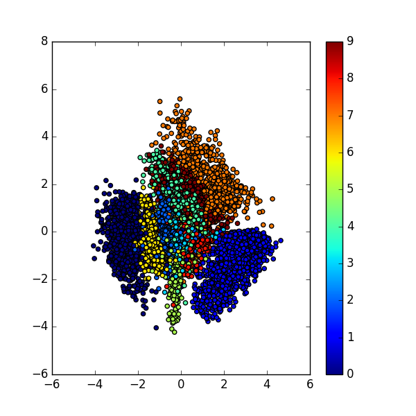
As we could see, in the latent space, the representation of our data that have the same characteristic, e.g. same label, are close to each other. Notice that in the training phase, we never provide any information regarding the data.
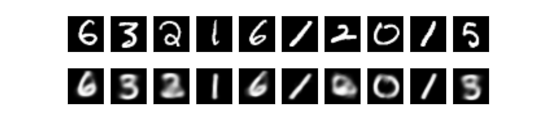
We could also look at the data reconstruction by running through the data into overall VAE net:
Lastly, we could generate new sample by first sample \( z \sim N(0, 1) \) and feed it into our decoder net:
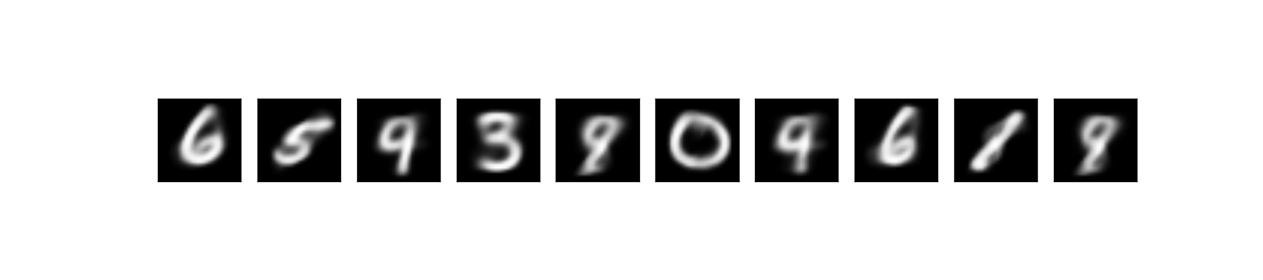
If we look closely on the reconstructed and generated data, we would notice that some of the data are ambiguous. For example the digit 5 looks like 3 or 8. That’s because our latent variable space is a continous distribution (i.e. \( N(0, 1) \)), hence there bound to be some smooth transition on the edge of the clusters. And also, the cluster of digits are close to each other if they are somewhat similar. That’s why in the latent space, 5 is close to 3.
Conclusion
In this post we looked at the intuition behind Variational Autoencoder (VAE), its formulation, and its implementation in Keras.
We also saw the difference between VAE and GAN, the two most popular generative models nowadays.
For more math on VAE, be sure to hit the original paper by Kingma et al., 2014. There is also an excellent tutorial on VAE by Carl Doersch. Check out the references section below.
References
- Doersch, Carl. “Tutorial on variational autoencoders.” arXiv preprint arXiv:1606.05908 (2016).
- Kingma, Diederik P., and Max Welling. “Auto-encoding variational bayes.” arXiv preprint arXiv:1312.6114 (2013).
- https://blog.keras.io/building-autoencoders-in-keras.html