Numerical Solution of Linear Algebraic
Equations with Direct Methods

Introduction

The most basic task in linear algebra, and perhaps in all of scientific computing, is to solve for the unknowns in a set of linear algebraic equations. Linear, algebraic equations occur in almost all branches of numerical analysis. But their most visible application in engineering is in the analysis of linear systems. Any system whose response is proportional to the input is deemed to be linear. Linear systems include structures, elastic solids, heat flow, seepage of fluids, electromagnetic fields and electric circuits. If the system is discrete, such as a truss or an electric circuit, then its analysis leads directly to linear algebraic equations.

In the case of a statically determinate truss, like the Eiffel tower which is a three-dimensional truss structure, the equations arise when the equilibrium conditions of the joints are written down. The unknowns $x_1, x_2,\ldots, x_n$ represent the forces in the members and the support reactions, and the constants $b_1, b_2,\ldots, b_n$ are the prescribed external loads. The behavior of continuous systems is described by differential equations, rather than algebraic equations. However, because numerical analysis can deal only with discrete variables, it is first necessary to approximate a differential equation with a system of algebraic equations. The well-known finite difference, finite element and boundary element methods of analysis work in this manner. They use different approximations to achieve the “discretization,” but in each case the final task is the same: solve a system (often a very large system) of linear, algebraic equations.

In summary, the modeling of linear systems invariably gives rise to equations of the form $\mathbf{A}.\mathbf{x} = \mathbf{b}$, where $\mathbf{b}$ is the input and $\mathbf{x}$ represents the response of the system. The coefficient matrix $\mathbf{A}$, which reflects the characteristics of the system, is independent of the input. In other words, if the input is changed, the equations have to be solved again with a different $\mathbf{b}$, but the same $\mathbf{A}$.

Therefore, it is desirable to have an equation solving algorithm that can handle any number of constant vectors with minimal computational effort. In general, a set of linear algebraic equations looks like this:

The $n$ unknowns $x_j$ , $j=1,\ldots,n$ are related by $m$ equations. The coefficients $a_{i,j}$ with $i=1,\ldots,m$ and $j=1,\ldots,n$ are known numbers, as are the right-hand side quantities $b_i$ with $i=1,\ldots,m$. If $n=m$ then there are as many equations as unknowns, and there is a good chance of solving for a unique solution set of $x_j$’s. Otherwise, if $n\neq m$, things are even more interesting; we’ll have more to say about this below. If we write the coefficients $a_{i,j}$ as a matrix, and the right-hand sides $b_i$ as a column vector the previous system can be written in matrix form as $\mathbf{A}.\mathbf{x}=\mathbf{b}$ where \[ \mathbf{A}=\left[ \begin{array} [c]{cccc}% a_{1,1} & a_{1,2} & \cdots & a_{1,n}\\ a_{2,1} & a_{2,2} & \cdots & a_{2,n}\\ \vdots & \vdots & & \vdots\\ a_{m,1} & a_{m,2} & \cdots & a_{m,n} \end{array} \right]. \] Throughout this page, we use a raised dot to denote matrix multiplication, or the multiplication of a matrix and a vector, or the dot product of two vectors.

With python, we will use the numpy library to deal with matrices. For instance, the following so called Wilson matrix \[ \mathbf{A}=\left[ \begin{array} [c]{cccc}% 10 & 7 & 8 & 7\\ 7 & 5 & 6 & 5\\ 8 & 6 & 10 & 9\\ 7 & 5 & 9 & 10 \end{array} \right] \] can be defined in python like this:

import numpy as np

""" Define the linear system elements: matrix  A and vector b """

A = np.array([[10, 7, 8, 7],[7, 5, 6, 5],[8, 6, 10, 9],[7, 5, 9, 10]])
b = np.array([1, 1, 1, 1])

We can also create a matrix by using some numpy functions

import numpy as np

A = np.zeros((3,3),dtype=np.float)
B = np.zeros((3,3),dtype=np.float64)

# Modification of the diagonal of matrix A
n = A.shape[0]
for i in range(n):
    A[i,i] = 2.0
print(A)

A particularly useful representation of the equations for computational purposes is the augmented coefficient matrix obtained by adjoining the constant vector $\mathbf{b}$ to the coefficient matrix $\mathbf{A}$ in the following fashion: $$ \left[\mathbf{A}|\mathbf{b}\right]= \left[ \begin{array}[c]{cccc} a_{1,1} & a_{1,2} & \cdots & a_{1,n}\\ a_{2,1} & a_{2,2} & \cdots & a_{2,n}\\ \vdots & \vdots & & \vdots\\ a_{m,1} & a_{m,2} & \cdots & a_{m,n} \end{array} \left| \begin{array}{c} b_1 \\ b_2 \\ \vdots \\ b_m \end{array}\right.\right] $$

For $m=n$, we can solve the unknows except when one or more of the $m$ equations is a linear combination of the others. We call this condition row degeneracy. When all equations contain certain variables only in exactly the same linear combination, we call this condition column degeneracy. It turns out that, for square matrices, row degeneracy implies column degeneracy, and vice versa. A set of equations that is degenerate is called singular.

Backsubstitution method

Exercice [PY-1]

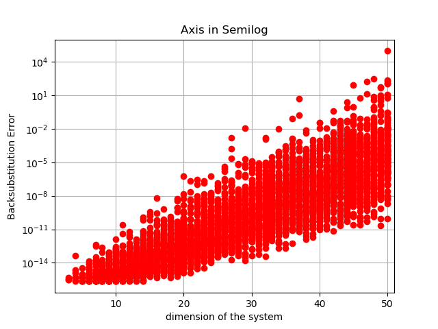
In this exercice we want to define the Backsubstitution function. For this, we need to know the dimension of the matrix by using the shape function. We assume that the matrix is a square matrix. We will also test the accuracy of the solution and consequently the sensibility of the method according to the dimension of the matrix.

1) Define the python Backsubstitution function. This function will return the $\mathbf{x}$ solution to the linear system $\mathbf{A}.\mathbf{x}=\mathbf{b}$ where $\mathbf{A}$ is assumed to be a upper triangular matrix.

                
import numpy as np

""" Definition of the Backsubstitution function """

def Backsubstitution(A,b):
    n = A.shape[0] 
    if b.shape[0] == n:
        x = np.zeros(n,dtype=np.float)
    
        for i in range(n-1,-1,-1):
            #TO DO 
            
    else:
        raise ValueError("shape index error")

    return x
    
# Use this function
A = np.array([[10, 7, 8, 7],[0, 5, 6, 5],[0, 0, 10, 9],[0, 0, 0, 10]])
b = np.array([1, 1, 1, 1])     
print(A)
print(b)
X = Backsubstitution(A,b)
print("Approximation solution of the system: ",X)
        
    

                            
def Backsubstitution(A,b):
    n = A.shape[0] 
    if b.shape[0] == n:
        x = np.zeros(n,dtype=np.float)

        for i in range(n-1,-1,-1):
            try:
                s = 0.0
                for j in range(n-1,i,-1):
                    s = s +  x[j]*A[i,j]
                x[i] = (b[i]-s)/A[i,i]
            except ZeroDivisionError:
                print("Error: Division by Zero")
            except IndexError:
                print("Error: index ",i," out of bounds")
    
    else:
        raise ValueError("shape index error")

    return x
                            
                        

2) In order to test the accuracy of the function, we define the coefficients of $\mathbf{A}$ by using a continuous uniform distribution on the interval $[-1,1]$. We also set the vector solution $x$ to $x=(1.0,..,1.0)^T$. By this way we are able to compare the exact solution $\mathbf{x}$ to the one obtained by using the Backsubstitution function according to different values of the dimension $n$ of the system.

            
# define a random matrix A

for i in range(n):
    for j in range(i,n):
        # select one random value according to the continuous 
        # uniform distribution on -1.0 and 1.0
        A[i,j] = np.random.uniform(-1.0,1.0,1)
        
# Create a vector with only "1"
x = np.ones(n,dtype=np.float)

# Calculate the associated vector b such that b=Ax        
b = np.dot(A,x)
    
X = Backsubstitution(A,b)

# Compare the exact solution x with X
# which is obtained by the use of the previous function
err = np.max(np.abs(x-X))
print("Max error of the solution = ",err)

        
    

The np.dot function allows to calculate the dot product of a matrix with a matrix or a vector.

                            
# create an empty list
ERR = []
# define the maximum dimension of the linear systems
dim = 50
# define the number of random system for each value of n
nb = 100

for n in range(1,dim+1):
    temp = []
    for k in range(nb):
        A = np.zeros((n,n),dtype=np.float)
        
        for i in range(n):
            for j in range(i,n):
                # select one random value according to the uniform distribution
                # on the interval -1.0 and 1.0
                A[i,j] = np.random.uniform(-1.0,1.0,1)
                
        # Create a vector with only "1"
        x = np.ones(n,dtype=np.float)

        b = np.dot(A,x)    
        X = Backsubstitution(A,b)
        err = np.max(np.abs(X-x))
        temp.append(err)
    ERR.append(temp)
                            
                        

                        
import matplotlib.pyplot as plt

# transpose the ERR list
ERR = np.transpose(ERR)

# Display grid
plt.grid(True, which="both")

# create a list of dim integer values
t = np.linspace(1,dim)

# Linear X axis, Logarithmic Y axis
for k in range(nb):
plt.semilogy(t,ERR[k],'ro')

#plt.ylim([0,1000])
plt.xlim([1,51])

# Provide the title for the semilog plot
plt.title('Axis in Semilog')

# Give x axis label for the semilog plot
plt.xlabel('dimension of the system')

# Give y axis label for the semilog plot
plt.ylabel('Backsubstitution Error')

# Display the semilog plot
plt.show()
#plt.savefig('BacksubstitutionErrors.png')
                        
                    

Gauss-Jordan elimination method

The idea behind Gauss-Jordan elimination is to use elementary row operations on the system that replace a system with an equivalent but simpler sytem for which the answers to the questions about solutions are "obvious". The Gauss elimination method needs three steps:

1. algebraic operations by swapping rows for successively eliminating the unknows which is similar to define an invertible matrix $\mathbf{M}$ such that matrix $\mathbf{M}.\mathbf{A}$ becomes an upper triangular matrix
2. calculating vector $\mathbf{M}.\mathbf{b}$
3. solving the linear system $\mathbf{M}.\mathbf{A}.\mathbf{x}=\mathbf{M}.\mathbf{b}$ where $\mathbf{M}.\mathbf{A}$ is a upper triangular matrix

By applying the backsubstitution algorithm we can then solve this linear system. In case one pivot is null, we search in which column we have a non-null pivot and we swap these columns. If it is impossible then we have $det(\mathbf{A})=0$.

for k=1 to n-1 do 
    if |akk| < eps then 
        Error Message
    else
        for i=k+1 to n do 
            c= aik/akk
            bi= bi - c bk 
            aik = 0
            for j = k+1 to n do 
                aij = aij - c.akj 
if |ann|< eps then  
    Error message             

Exercice [PY-2]

        
import numpy as np
import time


def GaussJordan(A,b, eps = 0.000001):
    n = A.shape[0]
    test = true
    # TO DO
    return test

n = 50

# select random values according to the uniform distribution
# between -1.0 and 1.0 for each coefficient of matrix A
A = np.random.uniform(-1.0,1.0,size=(n,n))
        
# Create a random vector according the uniform distribution
x = np.random.uniform(-1.0,1.0,n)
b = np.dot(A,x)


# Solve the linear system and give the calculation time needed to solve the system

start_time = time.time()
if GaussJordan(A,b):
    X = Backsubstitution(A,b)
    t =(time.time() - start_time)
    err = np.max(np.abs(X-x))
    print("n= ",n," time= ",t," err= ",err)
        
    

                        



def GaussJordan(A,b, eps = 0.000001):
    n = A.shape[0]
    test = True

    if b.shape[0] == n:    
        
    for k in range(n-1):
        try:
            if np.abs(A[k,k]) > eps:
                for i in range(k+1,n):
                    c = A[i,k]/A[k,k]
                    b[i] = b[i] - c * b[k]
                    A[i,k] = 0.0
                    for j in range(k+1,n):
                        A[i,j] = A[i,j] - c * A[k,j]
                else:
                    test = False
                    raise ValueError("Division by Zero")
                    
            except ZeroDivisionError:
                test = False
                print("Error: Division by Zero")
            except IndexError:
                test = False
                print("Error: index ",i," out of bounds")
            if np.abs(A[n-1,n-1]) < eps:
                    test = False
                    raise ValueError("Division by Zero")
        else:
        test = False
        raise ValueError("shape index error")
        
    return test
                        
                    

We assume now that we have a computer with three significative digits. If we solve the following linear system \[% \begin{array} [c]{r}% 10^{-4}x_{1}+x_{2}=1\\ x_{1}+x_{2}=2 \end{array} \] we obtain the 'exact' solutions: $x_{1}=1,00010...\;\;,\;x_{2}=0,99990...$

By applying the Gauss elimination method, we obtain \[% \begin{array} [c]{r}% x_{1}+10^{4}x_{2}=10^{4}\\ -9990x_{2}=-9990 \end{array} \] because $-10^{4}+1=-9999$ and $-10^{4}+2=-9998$ are roundoff to $-9990$. It yields \[ x_{1}\simeq0\text{ et }x_{2}\simeq1 \] If we swap the two rows: \[% \begin{array} [c]{r}% x_{1}+x_{2}=2\\ 10^{-4}x_{1}+x_{2}=1 \end{array} \] then we have: \[% \begin{array} [c]{r}% x_{1}+x_{2}=2\\ 0,999x_{2}=0,999 \end{array} \] Indeed, $-10^{-4}+1=0,9999\simeq0,999$ and $-2.10^{-4}+1=0,9998\simeq 0,999.$ It yields the more accurate values \[ x_{1}\simeq1\text{ et }x_{2}\simeq1 \] Consequently, by swaping rows or columns such that the "Gauss pivot" be the larger as possible, we can obtain a more accurate result.

Exercice [PY-3]

Cramer's rule

We are now going to derive explicit formulas for the solution of $\mathbf{A}x=\mathbf{b}$. The matrix $\mathbf{A}$ of this linear system is a square matrix of order $n$, and we shall assume that is not singular. We set \[ x_{i}=\frac{\det\left( \mathbf{B}_{i}\right) }{\det\left( \mathbf{A}\right) }% \] where \[ \mathbf{B}_{i}=\left[ \begin{array} [c]{ccccccc}% a_{11} & \cdots & a_{1,i-1} & b_{1} & a_{1,i+1} & \cdots & a_{1n}\\ a_{21} & \cdots & a_{2,i-1} & b_{2} & a_{2,i+1} & \cdots & a_{2n}\\ \vdots & & \vdots & \vdots & \vdots & & \vdots\\ a_{n1} & \cdots & a_{n,i-1} & b_{n} & a_{n,i+1} & \cdots & a_{nn}% \end{array} \right] \] We then calculate $n+1$ determinants and $n$ divisions. For calculating one determinant, we must do $n!-1$ additions, $n!(n-1)$ multiplications. This yields to: \begin{align*} & \left( n+1\right) !\text{ additions,}\\ & \left( n+2\right) !\text{ multiplications,}\\ & \text{and } n\text{ divisions.} \end{align*} For $n=10$ we need to do \begin{align*} & 900\;\text{operations for the Gauss elimination}\\ & 400\;000\;000\;\text{operations for the Cramer method}\\ & \text{No comment ....}% \end{align*}

Inverse of a matrix

There might be cases where the matrix is not invertible and then the system cannot be solved. Consider the following linear system of equations: $$\mathbf{A}=\left[\begin{array}{ccc} 1 & 1 & -1\\ 1 & -2 & 3\\ 2 & -1 & 2 \end{array}\right],\qquad\mathbf{b}=\left[\begin{array}{c} 1\\ -2\\ 3 \end{array}\right]$$ where only the last element of $\mathbf{A}$ changed. Let us try to apply the Gauss-Jordan elimination here: $$\mathbf{A}=\left[\begin{array}{ccc} 1 & 1 & -1\\ 1 & -2 & 3\\ 2 & -1 & 2 \end{array}\left|\begin{array}{ccc} 1 & 0 & 0\\ 0 & 1 & 0\\ 0 & 0 & 1 \end{array}\right.\right]$$ Operations 2 and 3: Multiply row 1 by -1 and sum to row 2: $$\mathbf{A}=\left[\begin{array}{ccc} 1 & 1 & -1\\ 0 & -3 & 4\\ 2 & -1 & 2 \end{array}\left|\begin{array}{ccc} 1 & 0 & 0\\ -1 & 1 & 0\\ 0 & 0 & 1 \end{array}\right.\right]$$ Operations 2 and 3: Multiply row 1 by -2 and sum to row 3: $$\mathbf{A}=\left[\begin{array}{ccc} 1 & 1 & -1\\ 0 & -3 & 4\\ 0 & -3 & 4 \end{array}\left|\begin{array}{ccc} 1 & 0 & 0\\ -1 & 1 & 0\\ -2 & 0 & 1 \end{array}\right.\right]$$ Consequently two rows are equal on the left side... Multiply row 2 by -1 and sum to row 3: $$\mathbf{A}=\left[\begin{array}{ccc} 1 & 1 & -1\\ 0 & -3 & 4\\ 0 & 0 & 0 \end{array}\left|\begin{array}{ccc} 1 & 0 & 0\\ -1 & 1 & 0\\ -1 & -1 & 1 \end{array}\right.\right]$$ We then lost one row. No matter the path we take, we will always have a zero-ed row in this case and cannot make the left side equal to the identity matrix. The reason for this is that any row in this matrix can be made by a linear combination of the other two (e.g. sum rows 1 and 2 of $\mathbf{A}$ and you get row 3). In other words, the system is really made from two equations and the other is generated by the original two rows. Then we have more variables than equations and the system cannot be solved. The fact that the matrix $\mathbf{A}$ cannot be inverted is a sign that the system is not solvable. In those situations, it is said the matrix is noninvertible or singular. We can also state that the rows of the matrix are linearly dependent, because we can make one by a linear combination of the others.

Now a piece of important trivia regarding matrix inversion:

• If a matrix is non-invertible, its transpose is non-invertible too
• From the previous, the columns of a non-invertible matrix are linearly dependent
• If the determinant of a matrix is zero, then the matrix is not invertible
• The rank of an invertible matrix of size $n\times n$ is $n$ (full rank)
• The eigenvalues of the an invertible matrix are all different from zero

• While not exact linear combinations of each other, some of the equations may be so close to linearly dependent that roundoff errors in the machine render them linearly dependent at some stage in the solution process. In this case your numerical procedure will fail, and it can tell you that it has failed.

• Accumulated roundoff errors in the solution process can swamp the true solution. This problem particularly emerges if $n$ is too large. The numerical procedure does not fail algorithmically. However, it returns a set of $x$’s that are wrong, as can be discovered by direct substitution back into the original equations. The closer a set of equations is to being singular, the more likely this is to happen, since increasingly close cancellations will occur during the solution. In fact, the preceding item can be viewed as the special case in which the loss of significance is unfortunately total.

Much of the sophistication of well-written linear equation-solving packages is devoted to the detection and/or correction of these two pathologies. It is difficult to give any firm guidelines for when such sophistication is needed, since there is no such thing as a “typical” linear problem. But here is a rough idea: Linear sets with $n$ no larger than $20$ or $50$ are routine if they are not close to singular; they rarely require more than the most straightforward methods, even in only single precision or float. With double precision, this number can readily be extended to $n$ as large as perhaps $1000$, after which point the limiting factor anyway soon becomes machine time, not accuracy. Even larger linear sets, $n$ in the thousands or millions, can be solved when the coefficients are sparse (that is, mostly zero), by methods that take advantage of the sparseness. Unfortunately, one seems just as often to encounter linear problems that, by their underlying nature, are close to singular. In this case, you might need to resort to sophisticated methods even for the case of $n=10$. Singular value decomposition is a technique that can sometimes turn singular problems into nonsingular ones, in which case additional sophistication becomes unnecessary.

There are many algorithms dedicated to the solution of large sets of equations, each one being tailored to a particular formof the coefficient matrix (symmetric, banded, sparse...). A well-known collection of these routines is LAPACK—Linear Algebra PACKage, originally written in Fortran77. The NumPy linear algebra functions rely on BLAS and LAPACK to provide efficient low level implementations of standard linear algebra algorithms. Those libraries may be provided by NumPy itself using C versions of a subset of their reference implementations but, when possible, highly optimized libraries that take advantage of specialized processor functionality are preferred (see numpy.linalg).

A system of $n$ linear equations in $n$ unknowns has a unique solution, provided that the determinant of the coefficient matrix is nonsingular; that is, $det(A)=0$. The rows and columns of a nonsingular matrix are linearly independent in the sense that no row (or column) is a linear combination of other rows (or columns). If the coefficient matrix is singular, the equations may have an infinite number of solutions, or no solutions at all, depending on the constant vector.

Let's say we have the following system of linear equations: $$\begin{array}{ccccc} x_{1} & +x_{2} & -x_{3} & = & 1\\ x_{1} & -2x_{2} & +3x_{3} & = & -2\\ -x_{1} & 2x_{2} & -x_{2} & = & 3 \end{array}$$ This can be represented in matrix form as: $$\mathbf{Ax=b},$$ where $$\mathbf{A}=\left[\begin{array}{ccc} 1 & 1 & -1\\ 1 & -2 & 3\\ -1 & 2 & -1 \end{array}\right],\qquad\mathbf{x}=\left[\begin{array}{c} x_{1}\\ x_{2}\\ x_{3} \end{array}\right],\qquad\mathbf{b}=\left[\begin{array}{c} 1\\ -2\\ 3 \end{array}\right].$$ To find $\mathbf{x}$, one needs to do the equivalent to divide $\mathbf{b}$ by $\mathbf{A}$. Since $\mathbf{A}$ is a matrix, we cannot simply divide by it. Instead, we make use of the notion of inverse of a matrix. The inverse of a matrix $\mathbf{A}$ is a matrix such that, when one is multiplied by the other, the result is the identity matrix $\mathbf{I}$ (a special matrix with 1's in the diagonal and 0's everywhere else): $$\mathbf{A^{-1}A=AA^{-1}=I}$$ In our original problem, we can then premultiply each side of the equation by the inverse of $\mathbf{A}$ to get: $$\mathbf{A^{-1}Ax=x=A^{-1}b}$$ To find this inverse, we need to find each element in the matrix $\mathbf{A^{-1}}$ that, when multiplied by the matrix $\mathbf{A}$, will produce the identity matrix. To do that, we can use the widely known Gauss-Jordan elimination method. We will use a joint matrix $\left[\mathbf{A|I}\right]$ by concatenating the columns of $\mathbf{A}$ and $\mathbf{I}$. Then, we perform a set of operations that converts $\mathbf{A}$ into $\mathbf{I}$. In the process, $\mathbf{I}$ is converted into $\mathbf{A^{-1}}$, concluding the joint matrix $\left[\mathbf{I|A^{-1}}\right]$. For our example: $$\mathbf{A}=\left[\begin{array}{ccc} 1 & 1 & -1\\ 1 & -2 & 3\\ -1 & 2 & -1 \end{array}\left|\begin{array}{ccc} 1 & 0 & 0\\ 0 & 1 & 0\\ 0 & 0 & 1 \end{array}\right.\right]$$ We can do the following operations to the joint matrix:

1. Swap two rows
2. Multiply a row by a non-zero scalar
3. Sum two rows and replace one of them with the result

Operation 3: Sum rows 2 and 3 and store the result in row 3: $$\mathbf{A}=\left[\begin{array}{ccc} 1 & 1 & -1\\ 1 & -2 & 3\\ 0 & 0 & 2 \end{array}\left|\begin{array}{ccc} 1 & 0 & 0\\ 0 & 1 & 0\\ 0 & 1 & 1 \end{array}\right.\right]$$ Operations 2 and 3: Multiply row 1 by -1, sum with row 2 and store result in 2: $$\mathbf{A}=\left[\begin{array}{ccc} 1 & 1 & -1\\ 0 & -3 & 4\\ 0 & 0 & 2 \end{array}\left|\begin{array}{ccc} 1 & 0 & 0\\ -1 & 1 & 0\\ 0 & 1 & 1 \end{array}\right.\right]$$ Operations 2 and 3: Multiply row 3 by -2, sum with row 2 and store result in 2: $$\mathbf{A}=\left[\begin{array}{ccc} 1 & 1 & -1\\ 0 & -3 & 0\\ 0 & 0 & 2 \end{array}\left|\begin{array}{ccc} 1 & 0 & 0\\ -1 & -1 & -2\\ 0 & 1 & 1 \end{array}\right.\right]$$ Operation 2: Multiply row 2 by -1/3 and row 3 by 1/2: $$\mathbf{A}=\left[\begin{array}{ccc} 1 & 1 & -1\\ 0 & 1 & 0\\ 0 & 0 & 1 \end{array}\left|\begin{array}{ccc} 1 & 0 & 0\\ 1/3 & 1/3 & 2/3\\ 0 & 1/2 & 1/2 \end{array}\right.\right]$$ Operations 2 and 3: Mutiply row 2 by -1 and sum to row 1, then sum row 3 to row 1: $$\mathbf{A}=\left[\begin{array}{ccc} 1 & 0 & 0\\ 0 & 1 & 0\\ 0 & 0 & 1 \end{array}\left|\begin{array}{ccc} 2/3 & 1/6 & -1/6\\ 1/3 & 1/3 & 2/3\\ 0 & 1/2 & 1/2 \end{array}\right.\right]$$ We end with the inverse: $$\mathbf{A^{-1}}=\left[\begin{array}{ccc} 2/3 & 1/6 & -1/6\\ 1/3 & 1/3 & 2/3\\ 0 & 1/2 & 1/2 \end{array}\right]$$ Now we can solve the system of equations at the beginning by $\mathbf{x=A^{-1}b}$. We could have solved the original problem by joining $\mathbf{A}$ and $\mathbf{b}$, and solving with the same method $\left[\mathbf{A|b}\right]$ (we would end up with $\left[\mathbf{I|x}\right]$). One of the benefit of calculating the inverse of $\mathbf{A}$ is that, in case we change $\mathbf{b}$, we only need to apply again $\mathbf{x=A^{-1}b}$ to solve the new system of equations.

To solve the inverse of a matrix $A$, we know that $A.A^{-1}=I$ where $I$ is the identity matrix. If we set $e_{i}$ the vector with null coordinates except the $i$-coordinate which is equal to $1$ then we can find the inverse matrix of $A$ by solving the $n$ following linear systems \begin{align*} A.X_{i} & =e_{i} \end{align*} where $X_{i}$ is the $i$-column of $A^{-1}$. To solve iteratively this inverse problem, we can use the $L.U$ decomposition method.

Let $L$ be a lower triangular matrix with $1$ on its diagonal and $U$ be a upper triangular matrix then with some assumptions matrix $A$ can be written as $A=L.U$. Hence, \begin{align*} Ax & =b\\ LUx & =b \end{align*} where, \[ A=\left[ \begin{array} [c]{cccc}% 1 & 0 & \ldots & 0\\ \times & 1 & & \vdots\\ \vdots & \ddots & \ddots & 0\\ \times & \cdots & \times & 1 \end{array} \right] \left[ \begin{array} [c]{cccc}% \times & \times & \ldots & \times\\ 0 & \times & & \vdots\\ \vdots & \ddots & \ddots & \times\\ 0 & \cdots & 0 & \times \end{array} \right] \] If we set $y=U.x$ then we firstly solve $L.y=b$ by using a forward substitution methodology. Hence, as we know the vector $y$, we can solve $U.x=y$ by using a back substitution method. Consequently, we finally obtain the unknow vector $x$. The main interest of this method is that if we have many linear systems with the same matrix $A$ we can use iteratively solve the systems with this $L.U$ decomposition. It can be obtained by using the Gauss elimination.

What is an ill-conditioned matrix?

Let us consider that the vector $\mathbf{b}$ is data collected by some sensors. This data comes with some error $\Delta\mathbf{b}$ attached to it. Our solution to the problem will be: $$\mathbf{x=A^{-1}(b+\Delta b)=A^{-1}b+A^{-1}\Delta b}=\mathbf{x^{\star}+A^{-1}\Delta b}$$ where $\mathbf{x^{\star}}$ is the true solution. The error of our solution caused by the error in the data is $$\mathbf{\Delta x=x-x^{\star}=A^{-1}\Delta b}$$ The error in $\mathbf{\Delta b}$ may get amplified by $\mathbf{A^{-1}}$ and produce a large error in $\mathbf{x}$. In those situations (where large error is a subjective criterion), we say the problem is ill-posed or ill-conditioned. Otherwise, the matrix is well-posed or well-conditioned. To make it simple, you can imagine $\mathbf{A}$ as a scalar $A$. If $\mathbf{A}$ is very small, then its inverse is very large. Then, even a small error in the data gets amplified by the large inverse of $\mathbf{A}$, producing a large deviation in the solution. For a pratical example: $$\mathbf{A}=\frac{1}{2}\left[\begin{array}{cc} 1 & 1\\ 1+10^{-10} & 1-10^{-10} \end{array}\right],\qquad\mathbf{A^{-1}}=\left[\begin{array}{cc} 1-10^{10} & 10^{10}\\ 1+10^{10} & -10^{10} \end{array}\right]$$ The problem with this matrix is that it is very close to being singular, although it is not. This is a condition of the problem and nothing can be done to solve it.

In order to evalute if a matrix is well-conditioned or not we need to introduce the matrix norm framework.
Let us recall that function $N$ is a norm on a vector space $E$ if \[ \left\{ \begin{array} [c]{l}% N:E\rightarrow\mathbb{R}^{+}\\ \forall x\in E\;\;N\left( x\right) =0\Leftrightarrow x=0\\ \forall x\in E\;\forall\lambda\in\mathbb{K}\;\;N\left( \lambda.x\right) =\left| \lambda\right| .N\left( x\right) \\ \forall x,y\in E\;\;N\left( x+y\right) \leq N\left( x\right) +N\left( y\right) \end{array} \right. \]

Definition. Let $N_{1}$ and $N_{2}$ be two norms on $E$. $N_{1}$ and $N_{2}$ are said equivalent iff \begin{align*} \exists\left( \alpha,\beta\right) & \in\left( \mathbb{R}^{+\ast}\right) ^{2}\; such\ that\\ \forall x & \in E\;\;\;\alpha N_{2}\left( x\right) \leq N_{1}\left( x\right) \leq\beta N_{2}\left( x\right) . \end{align*}

Theorem. if $E$ is a finite vector space then all norms on $E$ are equivalents.

Condition number of a linear system

Exercice [PY-4]

1) Define the Wilson matrix $\mathbf{A}$. For this, use the numpy and linalg python libraries.

        
import numpy as np
from numpy import linalg as LA

A=np.array([# To Do])
b=np.array([32,23,33,31])
c=np.array([32.1,22.9,33.1,30.9])
# Solve the linear system
x=LA.solve(A,b)
# solve the perturbated linear system
y=LA.solve(A,c)
print("Error : ",x-y)
        
    

2) Calculate the condition number of $\mathbf{A}$ for the $1$-norm and $2$-norm. For this, you need to create the following functions:

""" 1-Norm function """
def Norm1(A):
    #TO DO 
    return

""" 2-Norm function """
def Norm2(A):
    #TO DO 
    return value

Exercice [PY-5]

Define the Hilbert(n) function (see wikipedia for the definition of the Hilbert matrix) which allows to create the Hilbert matrix of dimension $n$. In this exercice, we want to show that this matrix is very ill-conditionned even for $n=5,10$ and $15$. We then solve the following linear system:

        
import numpy as np
from numpy import linalg as LA

""" Hilbert matrix function """
def Hilbert(n):
    #TO DO 
    return value

n=5
H=Hilbert(n)
x=np.ones(n)
b=np.dot(H,x)
X=LA.solve(H,b)

print("Error = ",x-X)

Exercice [AL-1]

Exercice [AL-2]

Exercice [AL-3]

The main objective of this exercice is to know how the solution $\mathbf{x}$ will be modified according to perturbations $\mathbf{\Delta A}$ of matrix $\mathbf{A}$ and $\mathbf{\Delta b}$ of vector $\mathbf{b}$ $$ (\mathbf{A} + \mathbf{\Delta A}).\mathbf{y}=\mathbf{b} + \mathbf{\Delta b} $$ where $\mathbf{\Delta A}\in \mathcal{M}_n(\mathbb{R})$ and $\mathbf{\Delta b}\in \mathbb{R}^n$. In this exercice we will consider a matrix norm induced by a vector norm of order $p$ (with $p \geq 1$). We also denote by $\mathbf{cond_p}(\mathbf{A})= \left\Vert \mathbf{A^{-1}}\right\Vert_p.\left\Vert \mathbf{A}\right\Vert_p$ the condition number of matrix $\mathbf{A}$.
Moreover, we assume that $\left\Vert \mathbf{A^{-1}}.\mathbf{\Delta A}\right\Vert_p \le 1$.

Linear Algebra framework

Let $\mathcal{L}\left( E,F\right) $ be the set of linear maps from $E$ to $F$. We can define the following operators in $\mathcal{L}\left( E,F\right) $:

Consequently $\mathcal{L}\left( E,F\right) $ is a vector space (also called linear space) in the field $\mathbb{K}$. If $E$ et $F$ are finite vector spaces then for any basis $\mathcal{B}% _{E}=\left( e_{j}\right) _{1\leq j\leq n}$ of $E$ and $\mathcal{B} _{F}=\left( f_{i}\right) _{1\leq i\leq m}$ of $F$, the linear map $g\in\mathcal{L}\left( E,F\right)$ is defined by the coefficients $\left( a_{ij}\right) $ such that: \[ g\left( e_{j}\right) =\sum_{i=1}^{m}a_{ij}f_{i}. \] We set these coefficients on the following table: \[ \begin{array}[c]{l|llll} & g\left( e_{1}\right) & g\left( e_{2}\right) & \cdots & g\left(e_{n}\right)\\ \hline f_{1} & a_{1,1} & a_{1,2} & \cdots & a_{1,n}\\ f_{2} & a_{2,1} & a_{2,2} & \cdots & a_{2,n}\\ \vdots & \vdots & \vdots & & \vdots\\ f_{m} & a_{m,1} & a_{m,2} & \cdots & a_{m,n} \end{array} \] where the values of the $j$-column of the table are the coordinates of the vector $g\left( e_{j}\right) $ in $\mathcal{B}_{F}$. Consequently, \[ A=\left( \begin{array} [c]{cccc}% a_{11} & a_{12} & \cdots & a_{1n}\\ a_{21} & a_{22} & \cdots & a_{2n}\\ \vdots & \vdots & & \vdots\\ a_{m1} & a_{m2} & \cdots & a_{mn}% \end{array} \right) , \]

is then called the $\bf{matrix}$ associated to the linear map $g\in \mathcal{L}\left( E,F\right)$ written in the basis $\left( e_{j}\right) _{1\leq j\leq n}$ and $\left( f_{i}\right) _{1\leq i\leq m}$. For all $x\in E$ such that $x=\sum\limits_{j=1}^{n}x_{j}e_{j}$, it yields

If $m$ is not equal to $n$ then matrix $A$ is rectangular. We denote by $\mathcal{M}_{m,n}\left( \mathbb{K}\right)$ the matrices set with $m$ rows and $n$ columns where all the coefficients belong to $\mathbb{K}$. $\mathcal{M}_{m,n}\left( \mathbb{K}\right) $, with the vector addition operator and the scalar multiplication on $\mathbb{K}$ is a vector space. We can show that the following matrices $E_{ij}=\left( e_{kl}\right) _{1\leq k\leq m,1\leq l\leq n}$ with $0$ coefficients except for $k=i$ and $l=j$ where $e_{kl}=1$ generate a basis for $\mathcal{M}_{m,n}\left( \mathbb{K}\right)$. The dimension of this space is then $mn.$

References

- P.G. Ciarlet (1982), Introduction à l’analyse numérique matricielle et à l’optimisation, Masson
- J.J. Dongarra, C.B. Moler, J.R. Bunch & G.W. Stewart (1979), LINPACK Users’ Guide. SIAM.
- D.K. Faddeev & V.N. Faddeeva (1963), Computational Methods of Linear Algebra. Freeman & Co.
- G.H. Golub & C.F. Van Loan (1989), Matrix Computations. Second edition. John Hopkins Univ. Press.
- N.J. Higham (1996), Accuracy and Stability of Numerical Algorithms. SIAM.
- A.S. Householder (1964), The Theory of Matrices in Numerical Analysis. Blaisdell Publ. Comp.
- G.W. Stewart (1973), Introduction to Matrix Computations. Academic Press.
- L.N. Trefethen & D. Bau (1997), Numerical Linear Algebra. SIAM.
- J.H. Wilkinson (1969), Rundungsfehler. Springer-Verlag.
- J.H. Wilkinson & C. Reinsch (1971), Handbook for Automatic Computation, Volume II, Linear Algebra. Springer-Verlag.