A Three Axis Plane Robot
Introduction
The main objective is to define the inverse kinematic model of the following three axis plane robot.
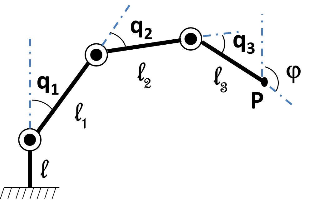 We assume that the different lengths $l,\ l_1,\ l_2$ and $l_3$ (given in millimeter) are the one of the UR 10 robot.
As soon as we know the joint angles $q_1,\ q_2$ and $\ q_3$ we can calculate with the direct geometric model
the position of the end effector $\textbf{P}$ and its orientation $\mathbf{\varphi}$. This orientation is calculated according to the vertical.
We assume that the different lengths $l,\ l_1,\ l_2$ and $l_3$ (given in millimeter) are the one of the UR 10 robot.
As soon as we know the joint angles $q_1,\ q_2$ and $\ q_3$ we can calculate with the direct geometric model
the position of the end effector $\textbf{P}$ and its orientation $\mathbf{\varphi}$. This orientation is calculated according to the vertical.
Direct Geometric Model
Linear Bezier parametric curve is obtained by linear interpolation between two given control points $\textbf{P}_0$ and $\textbf{P}_1$ in the plane.
$$ \text{For all } 0 \leq t \leq 1, \quad \mathcal{BP}\left[P_{0},P_{1}\right](t) = (1-t) \textbf{P}_0 + t \textbf{P}_1 $$Here, $\mathcal{BP}$, means Bezier Polynomial parametric curve. In the right window, you can see the basis polynomials of the linear Bezier curve. The red line is $(1-t)$ and the green one is $t$. In this example, the list of control points is $\textbf{P}$=[[0.1,0.1],[0.9,0.9]]
More generally, we have the following definition of Bezier curves:Quadratic Bezier curve
Quadratic Bezier curve is obtained from three control points $\textbf{P}_0$, $\textbf{P}_1$ and $\textbf{P}_2$. The Bezier curve is then defined by: $$ \text{For all } 0 \leq t \leq 1, \quad \mathcal{BP}\left[P_{0},P_{1},P_2\right](t) = B^2_0(t) \textbf{P}_0 + B^2_1(t) \textbf{P}_1 + B^2_2(t) \textbf{P}_2 $$ where the $B^2_0(t)=(1-t)^2$, $B^2_1(t)=2t(1-t)$ and $B^2_2(t)=t^2$ are the Bernstein polynomials of order $2$. They define a basis of the vector space of polynomials of degree less or equal to $2$. To the right you can see basis polynomials $B^2_0(t)$, $B^2_1(t)$ and $B^2_2(t)$ in the red, green and blue order.
By construction Bezier curve goes through its terminal control points ($\textbf{P}_0$ and $\textbf{P}_2$ here) and is tangent to the first and last segments of the control polygon. As we can, the Bezier curve "mimics" the shape of the control polygon. This can be possible due to the properties of the Bernstein polynomials. Usually, it is very difficult to design a polynomial curve when the curve is written in the canonical basis. This change of basis creates good visual conditions for "easy" design of the curves.
Cubic Bezier curve
In a similar way, for $n = 3$, we get a cubic Bezier curve
Bezier curve of degree $n = 7$
The initial control points are given by the following list:
$\textbf{P}$ = [[0.1,0.1],[0.1,0.8],[0.8,0.9],[0.8,0.2],[0.5,0.1],[0.3,0.5],[0.5,0.6],[0.9,0.3]]
On the right, we can see all the Bernstein polynomials $B^n_i(t)$ for $i=0,..,7$ needed to design this Bezier parametric curve.
By moving the control points (blue circles), you can see that the red curve, is always located in the convex hull of the control points of the Bezier curve. This property can be demonstrated.
Inverse Kinematic Model
In 1958, Paul Faget de Casteljau engineer at Citroën, developped a simple algorithm
which allows to calculate the value of $\mathcal{BP}(t)$ for any given value of $t$.
For example if $n = 2$ then his algorithm is defined as follows.
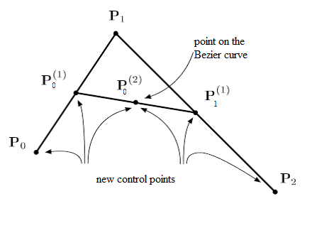
We fix the value of $t$ (for example $t=\dfrac{1}{2}$) and we calcute the two points $\textbf{P}^{(1)}_0$ and $\textbf{P}^{(1)}_1$ respectively the middle points of segments
$[\textbf{P}_0,\textbf{P}_1]$ and $[\textbf{P}_1,\textbf{P}_2]$.
They are calculated as follows for $t=\dfrac{1}{2}$:
\[
\begin{array}
[c]{l}%
\textbf{P}^{(1)}_0 = (1-t) \textbf{P}_0 + t \textbf{P}_1 \\
\textbf{P}^{(1)}_1 = (1-t) \textbf{P}_1 + t \textbf{P}_2 \\
\end{array}
\]
Finally, by iterating again this barycentric calcultation we obtain:
\[
\textbf{P}^{(2)}_0 = \textbf{BP}(t) = (1-t) \textbf{P}^{(1)}_0 + t \textbf{P}^{(1)}_1
\]
Note that $\textbf{P}^{(2)}_0$ subdivides the Bezier curve in two quadratic curves.
The new curves match the original in position, although they
differ in parameterization. The two polygons $[\textbf{P}_0,\textbf{P}^{(1)}_0,\textbf{P}^{(2)}_0]$
and $[\textbf{P}^{(2)}_0,\textbf{P}^{(1)}_1,\textbf{P}_2]$
are the control polygons of two new bezier curves that match perfectly the initial one.
In the following Figure, the two points $\textbf{P}^{(1)}_0$ and $\textbf{P}^{(1)}_1$ are the extremeties of the green segment and the point $\textbf{P}^{(2)}_0$ is the black point. They are calculated by the de Casteljau algorithm for different values of $t = \dfrac{i}{100}$ for $i=0,..,100$. Consequently, by joining all these black points it is possible to draw the Bezier curve in red. We then don't need to calculate the Bernstein polynoms.

More generally, Paul de Casteljau demonstrated the following theorem:
Exercice[de Casteljau Algorithm]
We want to draw a Bezier curve by using the de Casteljau algorithm.
-
Plot all the Bernstein polynomials for $n=3$. For this, use the following binomial function.
-
By using the result of the previous Theorem, implement the de Casteljau function for $j=n$. This function will return the value of $\mathcal{BP}(t)$ for a given $t$. $\textbf{P}$ is the list of the control points of the Bezier curve.
-
By using the previous decast function, draw the cubic Bezier curve with control polygon $\textbf{P}=[ [0.1,0.1],[0.9,0.9],[0.1,0.9],[0.9,0.1]]$. For this you can use a subdivision of $[0,1]$ by using np.linspace(0,1,100). Calculate for each values the corresponding values of the Bezier curve. The drawing of the Bezier curve is obtained by joining all these values. As in the previous Bezier examples you can draw also this control polygon.
    import numpy as np
    from math import factorial as fac

    def binomial(n,i):
        try:
            binom=fac(n)/(fac(i)*fac(n-i))
        except ValueError:
            binom=0.0
        return binom

    def bernstein(n,i,t):
        #TO DO
        return
        def bernstein(n,i,t):
            res=binomial(n,i)*(1-t)**(n-i)*t**i
            return res

        t=np.linspace(0,1,100)

        n=3
        for i in range(n+1):
            y=[bernstein(n,i,x) for x in t]
            plt.plot(t,y)
        plt.show()
    import numpy as np

    def decast(t,P):
        #TO DO
        return
        def decast(t,P):
            n=len(P)-1
            L0=P
            for k in range(n):
                L=L0
                L0=[]
                for i in range(n-k):
                    L0.append(np.dot(1-t,L[i])+np.dot(t,L[i+1]))
            return L0[0][0],L0[0][1]
    import numpy as np
    import matplotlib.pyplot as plt

    def DrawBezier(P,nb=100):
        #TO DO
        return
        def DrawBezier(P,nb=100):
            z=np.linspace(0,1,nb)
            X=[]
            Y=[]
            for t in z:
                x,y=decast(t,P)
                X.append(x)
                Y.append(y)
            return X,Y

        P=[[0.1,0.1],[0.9,0.9],[0.1,0.9],[0.9,0.1]]
        p=np.transpose(P)
        X,Y=DrawBezier(P)
        # Plot the control polygon of the Bezier curve
        plt.plot(p[0],p[1],'r')
        plt.plot(X,Y)
        plt.show()
References
- J.H. Ahlberg, E.N. Nilson & J.L. Walsh (1967) The Theory of Splines and Their Applications. Academic Press, New York.
- C. de Boor (1978) A Practical Guide to Splines. Springer-Verlag.
- G.D. Knott (2000) Interpolating Cubic Splines. Birkhäuser.
- H.J. Nussbaumer (1981) Fast Fourier Transform and Convolution Algorithms. Springer-Verlag.
- H. Späth (1995) One Dimensional Spline Interpolation. AK Peters.