Neural Networks for Datasets
Introduction
Gradient descent method is a way to find a local minimum of a function. The way it works is we start with an initial guess of the solution and we take the gradient of the function at that point. We step the solution in the negative direction of the gradient and we repeat the process. The algorithm will eventually converge where the gradient is zero (which correspond to a local minimum). Its brother, the gradient ascent, finds the local maximum nearer the current solution by stepping it towards the positive direction of the gradient. They are both first-order algorithms because they take only the first derivative of the function.
Let's say we are trying to find the solution to the minimum of some function $J(\mathbf{X})$. Given some initial value $\mathbf{X_0}$ for $\mathbf{X}$, we can change its value in many directions (proportional to the dimension of $\mathbf{X}$: with only one dimension, we can make it higher or lower). To figure out what is the best direction to minimize $J$, we take the gradient $\nabla J$ of it (the derivative along every dimension of $\mathbf{X}$). Intuitively, the gradient will give the slope of the curve at that $\mathbf{X}$ and its direction will point to an increase in the function. So we change $\mathbf{X}$ in the opposite direction to lower the function value: $$\mathbf{X}_{k+1} = \mathbf{X}_k - \lambda \nabla J(\mathbf{X}_k)$$ The $\lambda \gt 0$ is a small number that forces the algorithm to make small jumps. That keeps the algorithm stable and its optimal value depends on the function. Given stable conditions (a certain choice of $\lambda$), it is guaranteed that $J(\mathbf{X}_{k+1}) \le J(\mathbf{X}_k)$. There is a chronical problem to the gradient descent. For functions that have valleys (in the case of descent) or saddle points (in the case of ascent), the gradient descent/ascent algorithm zig-zags, because the gradient is nearly orthogonal to the direction of the local minimum in these regions. It is like being inside a round tube and trying to stay in the lower part of the tube. In case we are not, the gradient tells us we should go almost perpendicular to the longitudinal direction of the tube. If the local minimum is at the end of the tube, it will take a long time to reach it because we keep jumping between the sides of the tube (zig-zag). The Rosenbrock function is used to test this difficult problem.
Exercise [A "good" example]
We want to find the minimum value of the following function:
$$
J\left(x_{1},x_{2}\right)=\left(x_{1}^{2}-4x_{1}+4\right)\left(x_{1}^{2}+4x_{1}+2\right)
$$
-
Calculate the minimum values of this function.
We calculate the gradient vector of $J$. It yields: $$ \nabla J\left(x_1,x_2\right) = \left[\begin{array}{c} 4x_1^3-20x_1+8\\ 0\\ \end{array}\right] $$ Consequently, the possible minimum values are $2$, $\sqrt{2}-1$ or $-\sqrt{2}-1$.
We then calculate the hessian matrix: $$ \nabla^2 J\left(x_1,x_2\right) = \left[\begin{array}{cc} 12x_1^2-20 & 0\\ 0 & 0\\ \end{array}\right] $$ The hessian matrix is only positive definite for $x_1=2$ or $x_1=-\sqrt{2}-1$ whatever the value of $x_2$. -
Draw the level sets of the function. For this, you can use the following Python code:
import numpy as np import matplotlib.pyplot as plt """ Level sets""" def g(x1,x2): res = (x1**2-4*x1+4)*(x1**2+4*x1+2) return res # level set drawing of the function X1,X2 = np.meshgrid(np.linspace(-4,4,401),np.linspace(-3,2.5,401)) Z = g(X1,X2) graphe = plt.contour(X1,X2,Z,120) plt.show() -
Define the J and GradJ functions that allows to calculate the gradient of $J$ and the Hess which returns the hessian matrix of $J$.
import numpy as np import matplotlib.pyplot as plt """ The J, GradJ and Hess functions""" def J(X): res = (X[0]**2-4*X[0]+4)*(X[0]**2+4*X[0]+2) return res def GradJ(X): res = np.array([4*X[0]**3-20*X[0]+8.0, 0.0]) return res def Hess(X): res = np.array([[#TO DO,#TO DO],[#TO DO,#TO DO]]) return res -
Gradient Descent with a fixed $\lambda$ coefficient:
Let $X_{0}=\left(x_{1},x_{2}\right)=\left(-1,1\right)$ be the initial value. Calculate the $X_{k}$ values by using the following algorithm:
$k=0$
While $\left\Vert \nabla J\left(X_{k}\right)\right\Vert >\epsilon$
$\;\;\;\;\;\;\;\Delta=-\lambda.\nabla J(X_{k})$
$\;\;\;\;\;\;\;X_{k+1}=X_{k}+\Delta$
$\;\;\;\;\;\;\;k=k+1$
return $X_{k}$
Tune the value of $\lambda$.import numpy as np from numpy import linalg as LA import matplotlib.pyplot as plt """ The Gradient Descent function""" def Gradient(X0,lambda,eps,niter): k=0 while(#TO DO): #TO DO return x,y X0=[-1.0,1.0] lambda = 0.01 eps = 0.001 niter = 150 x0,y0 = Gradient(X0,lambda,eps,niter) plt.plot(x0,y0,'r', label=r"Gradient Method with a fixed $\lambda$", linestyle='--') plt.legend(loc='upper left', bbox_to_anchor=(1.1, 0.95),fancybox=True, shadow=True) plt.show() -
Draw the $X_{k}$ values of this algorithm in the level sets graph.
-
Confirm that the value found by the Algorithm is a local minimum value.
-
Gradient Descent with momentum:
Let $X_{0}=\left(-1,1\right)$ be the initial value. Calculate the $X_{k}$ values by using the following momentum Gradient Descent algorithm:
$\Delta=$0, $k=0$
While $\left\Vert \nabla J\left(X_{k}\right)\right\Vert >\epsilon$
$\;\;\;\;\;\;\;\Delta=-\lambda.\nabla J(X_{k})+\mu.\Delta$
$\;\;\;\;\;\;\;X_{k+1}=X_{k}+\Delta$
$\;\;\;\;\;\;\;k=k+1$
return $X_{k}$""" The Momentum Gradient Descent function""" def MGradient(X0,lambda,mu,eps,niter): k=0 while(#TO DO): #TO DO return x,y X0=[-1.0,1.0] lambda = 0.01 mu = 0.01 eps = 0.001 niter = 150 x1,y1 = MGradient(X0,lambda,mu,eps,niter) plt.plot(x1,y1,'r', label=r"Momentum Gradient Method") plt.legend(loc='upper left', bbox_to_anchor=(1.1, 0.95),fancybox=True, shadow=True) plt.show()
The $\mu\in\left[0,1\right[$ value has been to be tuned. -
Draw the $X_{k}$ values of this algorithm in the level sets graph.
-
Confirm that the value found by the Algorithm is a local minimum value.
""" The Gradient Descent function"""
def Gradient(X0,lambda,eps,niter):
    k=0
    LX=[X[0]]
    LY=[X[1]]
    while((LA.norm(GradJ(X))>eps and k< niter):
        X=X-np.dot(alpha,GradJ(X))
        k=k+1
        LX.append(X[0])
        LX.append(X[1])
    print("\n iteration number of the fixed step gradient descent method: ",k)
    print("Optimal value x= ",X[0]," y= ",X[1])
    return LX,LY
""" The Momentum Gradient Descent function"""
def MGradient(X0,lambda,mu,eps,niter):
    k=0
    LX=[X[0]]
    LY=[X[1]]
    Delta=[0.0 for i in range(len(X))]
    while((LA.norm(GradJ(X))>eps and k< niter):
        Delta=-np.dot(alpha,GradJ(X))+np.dot(beta,Delta)
        X=np.add(X,Delta)
        k=k+1
        LX.append(X[0])
        LX.append(X[1])
    print("\n iteration number of the gradient descent with momentum: ",k)
    print("Optimal value x= ",X[0]," y= ",X[1])
    return LX,LY
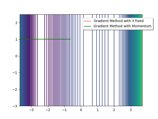
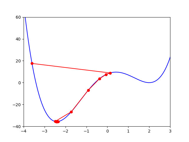
We obtain:
-
$7$ iterations of the Gradient Descent with $\lambda=0.02$ give:
x= -2.4141942582083296 and y= 1.0 -
$12$ iterations of the Momentum Gradient with $\lambda=0.02$ and $\mu=0.06$ give:
x= -2.4142172250611096 and y= 1.0
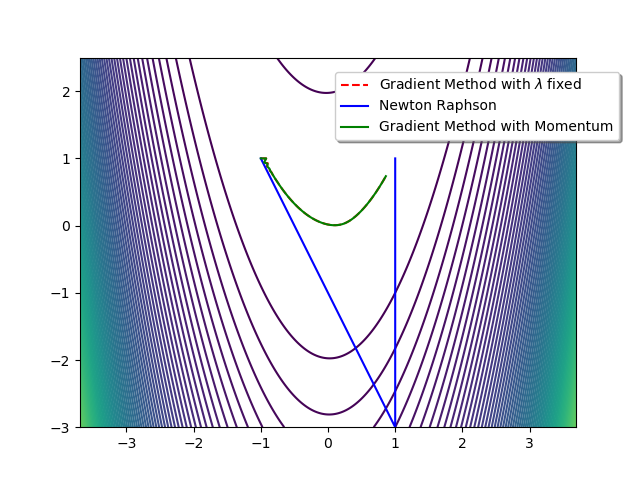
We want to find the minimum value of the following function: $$ J\left(x_{1},x_{2}\right)=\left(x_{1}-1\right)^{2}+10\left(x_{1}^{2}-x_{2}\right)^{2} $$
- Calculate the minimum value of this function.
-
Draw the level sets of this function.
-
Apply the previous Gradient Descent methods
-
Apply the Newton-Raphson Algorithm to this function.
""" The Newton-Raphson function"""
def Newton(X0,eps,niter):
    k=0
    x=[X[0]]
    y=[X[1]]
    while(LA.norm(GradJ(X))>eps and k< niter):
        delta=#TO DO
        X=X-delta
        k=k+1
        x.append(X[0])
        y.append(X[1])
    return x,y

X0=[-1.0,1.0]
eps = 0.001
niter = 150
x3,y3 = Newton(X0,eps,niter)
plt.plot(x3,y3,'r', label=r"Newton-Raphson Method")
plt.legend(loc='upper left', bbox_to_anchor=(1.1, 0.95),fancybox=True, shadow=True)
plt.show()
    import numpy as np

    """ GradJ and Hess functions"""

    def GradJ(X):
        res = np.array([2*(X[0]-1)+40*X[0]*(X[0]**2-X[1]),-20*(X[0]**2-X[1])])
        return res

    def Hess(X):
        res = np.array([[2 + 80*X[0]**2 + 40*(X[0]**2 - X[1]),-40*X[0]],[-40*X[0], 20]])
        return res

    """ The Newton-Raphson function"""
        delta=LA.solve(Hess(X),GradJ(X))
We obtain:
-
$150$ iterations of the Gradient Descent with $\lambda=0.02$ give:
x= 0.8467914701456682 y= 0.7102982431003074 -
$150$ iterations of the Momentum Gradient with $\lambda=0.02$ and $\mu=0.06$ give:
x= 0.8610575985931694 y= 0.73534414819584 -
$2$ iterations of the Newton Raphson method give:
x= 0.9999999999999982 y= 0.9999999999999964
Estimating the step-size
A wrong step size $\lambda$ may not reach convergence, so a careful selection of the step size is important. Too large it will diverge, too small it will take a long time to converge. One option is to choose a fixed step size that will assure convergence wherever you start gradient descent. Another option is to choose a different step size at each iteration (adaptive step size).
Any differentiable function has a maximum derivative value, i.e., the maximum of the derivatives at all points. If this maximum is not infinite, this value is known as the Lipschitz constant and the function is Lipschitz continuous. $$\frac{\left\Vert f(\mathbf{x})-f(\mathbf{y}) \right\Vert}{\left\Vert \mathbf{x} - \mathbf{y} \right\Vert}\le L(f), \textrm{ for any } \mathbf{x},\mathbf{y} $$ This constant is important because it says that, given a certain function, any derivative will have a smaller value than the Lipschitz constant. The same can be said for the gradient of the function: if the maximum second derivative is finite, the function is Lipschitz continuous gradient and that value is the Lipschitz constant of $\nabla f$. $$\frac{\left\Vert \nabla f(\mathbf{x})-\nabla f(\mathbf{y}) \right\Vert}{\left\Vert \mathbf{x} - \mathbf{y} \right\Vert}\le L(\nabla f), \textrm{ for any } \mathbf{x},\mathbf{y} $$ For the $f(x) = x^2$ example, the derivative is $df(x)/dx = 2x$ and therefore the function is not Lipschitz continuous. But the second derivative is $d^2f(x)/dx^2 = 2$, and the function is Lipschitz continuous gradient with Lipschitz constant of $\nabla f = 2$.
Each gradient descent can be viewed as a minimization of the function: $$\mathbf{x}_{k+1} = \underset{\mathbf{x}}{\arg\min} f(\mathbf{x}_k) + (\mathbf{x} - \mathbf{x}_k)^T\nabla f(\mathbf{x}_k) + \frac{1}{2\lambda}\left\Vert\mathbf{x} - \mathbf{x}_k\right\Vert^2 $$ If we differentiate the equation with respect to $\mathbf{x}$, we get: $$0 = \nabla f(\mathbf{x}_k) + \frac{1}{\lambda}(\mathbf{x} - \mathbf{x}_k)$$ $$\mathbf{x} = \mathbf{x}_k - \lambda\nabla f(\mathbf{x}_k)$$ It can be shown that for any $\lambda \le 1/L(\nabla f)$: $$f(\mathbf{x}) \le f(\mathbf{x}_k) + (\mathbf{x} - \mathbf{x}_k)^T\nabla f(\mathbf{x}_k) + \frac{1}{2\lambda}\left\Vert\mathbf{x} - \mathbf{x}_k\right\Vert^2 $$ i.e., for any $\mathbf{x}$, $f(\mathbf{x})$ will always be equal or lower than the function that the gradient descent minimizes, if $\lambda \le 1/L(\nabla f)$. Under this view, the result we get from minimizing the right hand side is an upper bound to the real value of the function at $\mathbf{x}$. In our good example above, $L(\nabla f) = 2$, then $\lambda \le 0.5$ for good convergence. In fact, for this simple case, $\lambda = 0.5$ is a perfect value for the step size: smaller will converge slower, larger will exceed the optimum point at each iteration (although it still converges up to $\lambda = 1$).
Adaptive step size
There are methods, known as line search, that make an estimate of what the step size should be at a given iteration. After calculating the gradient, these methods choose a step size by minimizing a function of the step size itself: $$\lambda_k = h(\lambda)$$Each method defines its own function, based on some assumptions. Exact methods accurately minimize $h(\lambda)$, while inexact methods make an approximation that just improves on the last iteration. The following are just a few examples.
Cauchy
One of the most obvious choices of $\lambda$ is to choose the one that minimizes the objective function: $$\lambda_k = \underset{\lambda}{\arg\min} f(\mathbf{x}_k - \lambda \nabla f(\mathbf{x}_k)) $$ This approach is conveniently called the steepest descent method. Although it seems to the best choice, it converges only linearly (error $\propto 1/k$) and is very sensitive to ill-conditioning of problems.
Barzilai and Borwein
An approach proposed in 1988 is to find the step size that minimizes: $$\lambda_k = \underset{\lambda}{\arg\min} \left\Vert \Delta\mathbf{x} - \lambda \Delta g(\mathbf{x}) \right\Vert^2$$ where $\Delta\mathbf{x} = \mathbf{x}_k - \mathbf{x}_{k-1}$ and $\Delta g(\mathbf{x}) = \nabla f(\mathbf{x}_k) - \nabla f(\mathbf{x}_{k-1})$. This is an approximation to the secant equation, used in quasi-Newton methods. The solution to this problem is easily solved differentiating with respect to $\lambda$: $$0 = \Delta g(\mathbf{x})^T (\Delta\mathbf{x} - \lambda \Delta g(\mathbf{x})) $$ $$\lambda = \frac{\Delta g(\mathbf{x})^T \Delta\mathbf{x}}{\Delta g(\mathbf{x})^T\Delta g(\mathbf{x})} $$ This approach works really well, even for large dimensional problems.
Backtracking
This is considered an inexact line search, in the sense it does not optimize $\lambda$, but instead chooses one that guarantees some descent.
Start with $\lambda > 0$ and $\tau \in (0,1)$.
Repeat $\lambda = \tau \lambda$
Until the Armijo-Goldstein or Wolfe conditions are met
Descent Lemma
In Proposition A.24 from Bertsekas 1999 we have the following result:
Proof.
$$f(\mathbf{x}+\mathbf{y})-f(\mathbf{x}) = \left.f(\mathbf{x}+t\mathbf{y})\right|_{t=1}-\left.f(\mathbf{x}+t\mathbf{y})\right|_{t=0}$$ The two terms can be seen as the limits of an integral: $$ \left.f(\mathbf{x}+t\mathbf{y})\right|_{t=1}-\left.f(\mathbf{x}+t\mathbf{y})\right|_{t=0} = \int_{0}^{1}\frac{df(\mathbf{x}+t\mathbf{y})}{dt}dt=\int_{0}^{1}\mathbf{y}^{T}\nabla f(\mathbf{x}+t\mathbf{y})dt$$ Let's add positive and negative versions of the same term: $$\int_{0}^{1}y^{T}\nabla f(\mathbf{x}+t\mathbf{y})dt = \int_{0}^{1}\mathbf{y}^{T}\nabla f(\mathbf{x}+t\mathbf{y}) - \mathbf{y}^{T}\nabla f(\mathbf{x}) dt + \int_{0}^{1} \mathbf{y}^{T}\nabla f(\mathbf{x}) dt$$ and take the norm of the first term, which guarantees the result is equal or greater than the original: $$f(\mathbf{x}+\mathbf{y}) - f(\mathbf{x}) \le \int_{0}^{1}\left\Vert\mathbf{y}^{T}(\nabla f(\mathbf{x}+t\mathbf{y}) - \nabla f(\mathbf{x})) \right\Vert_2dt + \int_{0}^{1} \mathbf{y}^{T}\nabla f(\mathbf{x}) dt$$ Now we make use of the Hölder's inequality $\left\Vert \mathbf{x}^T\mathbf{y} \right\Vert \le \left\Vert \mathbf{x} \right\Vert \left\Vert \mathbf{y} \right\Vert$: $$f(\mathbf{x}+\mathbf{y}) - f(\mathbf{x}) \le \left\Vert\mathbf{y}\right\Vert_2 \int_{0}^{1}\left\Vert\nabla f(\mathbf{x}+t\mathbf{y}) - \nabla f(\mathbf{x})\right\Vert_2 dt + \mathbf{y}^{T}\nabla f(\mathbf{x}) \int_{0}^{1} dt$$ Now we make use of the condition in the lemma to simplify the inequality: $$ f(\mathbf{x}+\mathbf{y}) - f(\mathbf{x}) \le \left\Vert\mathbf{y}\right\Vert_2 L \int_{0}^{1} t\left\Vert \mathbf{y} \right\Vert_2 dt + y^{T}\nabla f(\mathbf{x}) = \frac{L}{2}\left\Vert\mathbf{y}\right\Vert_2^2 + y^{T}\nabla f(\mathbf{x}). $$
References
- D. P. Bertsekas (1999), Nonlinear Programming.
- J. Barzilai, J.M. Borwein (1988), Two-Point Step Size Gradient Methods, IMA Journal of Numerical Analysis (8), pp. 141-148.