$$ \newcommand{\dint}{\mathrm{d}} \newcommand{\vphi}{\boldsymbol{\phi}} \newcommand{\vpi}{\boldsymbol{\pi}} \newcommand{\vpsi}{\boldsymbol{\psi}} \newcommand{\vomg}{\boldsymbol{\omega}} \newcommand{\vsigma}{\boldsymbol{\sigma}} \newcommand{\vzeta}{\boldsymbol{\zeta}} \renewcommand{\vx}{\mathbf{x}} \renewcommand{\vy}{\mathbf{y}} \renewcommand{\vz}{\mathbf{z}} \renewcommand{\vh}{\mathbf{h}} \renewcommand{\b}{\mathbf} \renewcommand{\vec}{\mathrm{vec}} \newcommand{\vecemph}{\mathrm{vec}} \newcommand{\mvn}{\mathcal{MN}} \newcommand{\G}{\mathcal{G}} \newcommand{\M}{\mathcal{M}} \newcommand{\N}{\mathcal{N}} \newcommand{\S}{\mathcal{S}} \newcommand{\diag}[1]{\mathrm{diag}(#1)} \newcommand{\diagemph}[1]{\mathrm{diag}(#1)} \newcommand{\tr}[1]{\text{tr}(#1)} \renewcommand{\C}{\mathbb{C}} \renewcommand{\R}{\mathbb{R}} \renewcommand{\E}{\mathbb{E}} \newcommand{\D}{\mathcal{D}} \newcommand{\inner}[1]{\langle #1 \rangle} \newcommand{\innerbig}[1]{\left \langle #1 \right \rangle} \newcommand{\abs}[1]{\lvert #1 \rvert} \newcommand{\norm}[1]{\lVert #1 \rVert} \newcommand{\two}{\mathrm{II}} \newcommand{\GL}{\mathrm{GL}} \newcommand{\Id}{\mathrm{Id}} \newcommand{\grad}[1]{\mathrm{grad} \, #1} \newcommand{\gradat}[2]{\mathrm{grad} \, #1 \, \vert_{#2}} \newcommand{\Hess}[1]{\mathrm{Hess} \, #1} \newcommand{\T}{\text{T}} \newcommand{\dim}[1]{\mathrm{dim} \, #1} \newcommand{\partder}[2]{\frac{\partial #1}{\partial #2}} \newcommand{\rank}[1]{\mathrm{rank} \, #1} $$
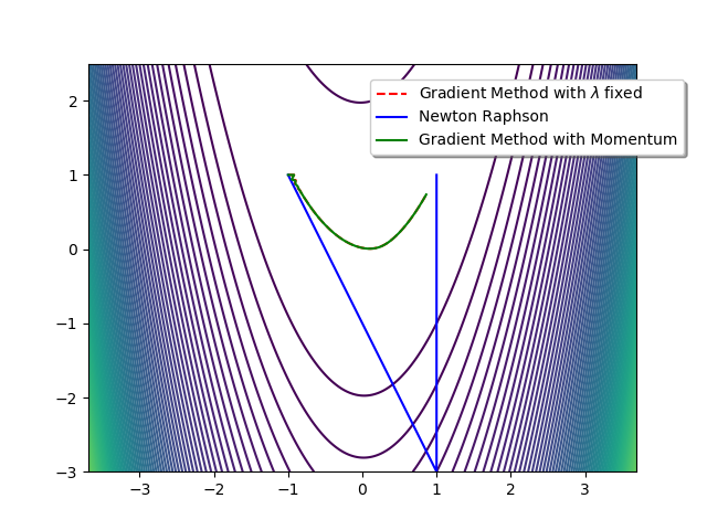
Different gradient methods are given for nonlinear optimization.
Posted by ogi on November 4, 2019
Posted by ogi on October 20, 2019
Posted by ogi on April 6, 2020