Supervised Classification
- Introduction
- K-nearest neighbors Algorithm
- Cross Validation and Parameters Selection
- Perceptron
- Support Vector Machine (SVM)
Introduction
The most classic example to introduce the concept of supervised learning is the one of apples and oranges. Fruits, that can be either apples or oranges, are transported on a conveyor belt. At the end of this conveyor belt, the fruit can be placed in one of two trays, and the goal is to sort the fruits according to their types. We want to automate the process of fruits classification, and one possible choice to do this is by using supervised machine learning methods.
 The core idea is fairly simple, all that is required is to gather a certain amount of labelled examples (for which the class is known) and use them to train a classification model. The training phase consists in using the example smartly, such that the parameters of the model built makes a good match between the example inputs and outputs (which are known). Such a model can then be used to predict the class of a new fruit that was never seen before.
To carry out such a supervised learning process, several steps need to be executed:
-
Reduce the problem to a numerical problem. Indeed, to create a mathematical model able to distinguish apples from oranges, the first step consists in converting the abstract concept of a fruit into a vector of numbers. The different components of such vector are called features. Choosing a feature vector is not an easy task in general, there can be several levels of abstraction in the choice of the features. For example, for the fruit classification problem, features can be high level (diameter of the fruit, weight, texture, ...) but it could also be a way more abstract representation (pixels of a picture of the fruit). The more abstract the representation is, the more examples are required to get a good classification model.
-
Once the objects to classify have been written in the form of $N$ features, they are expressed in a $N$ dimensional space called feature space. The second step in a classification algorithm is to partition such space in order to separate objects according to their classes. For instance, if any fruit is represented by its diameter and its weight, to any point in this two dimensional space the model should associate a class: apple or orange. This step is called learning, the goal is to tune the model such that it matches the observations provided by the labelled examples, that are also called training data.
-
The final step is called inference, or prediction. It simply consists in using the model obtained from the learning phase. Given a new object, represented by features and for which the class is unknown, the model needs to predict the class of this object.
- Medical diagnosis
- Amazon, Criteo (Web advertising)
- Microsoft, failure prediction and preventive maintenance
K-nearest neighbors Algorithm
This first algorithm is a good way to get started with machine learning because of its simplicity and very intuitive principle. The model is the database of inputs/outputs itself. When facing a new point, for which the class is unknown, the algorithm looks for the $k$ points in the dataset that are closest to this new feature vector. Then, the class attributed to the new object is the most represented class among the $k$ nearest neighbors. In general, the distance used to determine the nearest neighbors is the euclidean distance in the $N$ dimensional feature space, but in theory, such distance can be defined by any norm on the input space.
For instance, the following figure shows a Supervised classification problem in 2D.
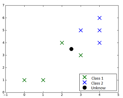 The eight points in green and blue represent the training set, the black point is a new data, of unknown class which should be predicted. The four figures that follow show the classification results using the K-nearest neighbors algorithm with different values of $k$.
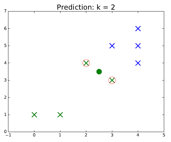
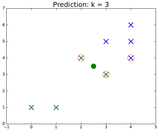
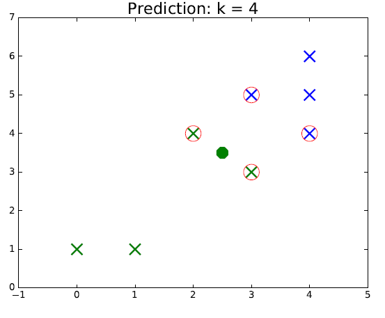
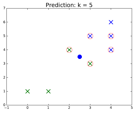
Looking at figure, it is rather intuitive to understand how this algorithm works. The points circled in red represent the selected neighbors for classification. The color of the new point represents the predicted class. We can see that as the green class is more spread out, if $k$ is chosen too large, it is possible make mistakes if we assume the "true" sets are separated by a line for example. Thus, the hyperparameter $k$ should be chosen carefully for each problem.
Exercise[Code the K-nearest neighbors algorithm]
-
We use the following data points from the picture data=[[0,1],[1,1],[3,3],[2,4],[4,4],[4,5],[4,6],[3,5]]. We associate to each data point its class by using the list target = [0,0,0,0,1,1,1,1]. Consequently, [0,1] has the 0 (or green) class and [4,5] has the 1 (blue) class.
Define the knn(P,data,target,k) python function. By using the $k$-nearest neighbors algorithm, this function will return for $k = 1$, $k=2$ or $k=3$ the class associated to a given data point P. For $k=1$, the class of the given point is the same than the training point that is closest to it. For $k=3$, you have to calculate the $3$-closest points and their class. For example, if we obtain the classes $0,0$ and $1$, the class result will be $0$. For this, you can use the following python code.import numpy as np # inputs data=[[0,1],[1,1],[3,3],[2,4],[4,4],[4,5],[4,6],[3,5]] target = [0,0,0,0,1,1,1,1] # define the distance function def distance(P,Q): res= np.sqrt((Q[0]-P[0])**2+(Q[1]-P[1])**2) return res # test this function print(distance([1,1],[5,3])) # define the k-nearest neighboors function for any value of k def knn(P,data,target,k): # TO DO return 0 # Test the function for a given data point P P = [2.5,3.5] print("The class of point ",P," is : ",knn(P,data,target,3)) -
Test it on the Iris dataset. This data sets consists of $3$ different types of irises: Setosa, Versicolour, and Virginica. The data are stored in a 150x4 numpy.ndarray. The rows being the samples and the columns being: Sepal Length, Sepal Width, Petal Length and Petal Width.
- Same question for any value of $k$.
-
import numpy as np
import time

### Useful tips ###
# To comment a block of lines, just highlight them and press 'ctrl + 1'
# When you don't know how to do something in programming, very often Google knows!

### Lists ###

print 'Lists:'
my_list_of_integers = [1, 2, 3] #Create a list, items can be of any type
my_list_of_strings  = ['abc', 'def']
my_mixed_type_list  = ['abc', 2, 21.3, 'def']

print ('first item of string list :', my_list_of_strings[0] #In python, starting index for a list is 0)
print ('last item of string list :', my_list_of_strings[-1] #A list can be indexed backward)
print ('Middle items of mixed list:', my_mixed_type_list[1:3] #By doing 1:3, & is taken but three is not included in the interval)

### Loops ###

print ('\nLoops:')
print ('types of mixed list items:')
for i in range(len(my_mixed_type_list)):#range(n) means that i loops from 0 to n-1
    print ('type of item ' + str(i), type(my_mixed_type_list[i]))

print ('\nprint all integers less than 3:')
k = 0
while k < 3:
    print(k)
    k += 1

### If statement ###

print ('\nIf statement:')
i = 3
if i == 2:
    print (str(i) + ' is equal to 2')
else:
    print (str(i) + ' is not equal to 2')

### Fonctions ###

print ('\nFunctions:')
def addition(x, y):
    return x + y
print ('5 + 6 is equal to :', addition(5, 6))

### Vecteurs et matrices ###

print ('\nVectors and Matrices:')
my_vector = np.array([0, 1, 2, 4])
print ('my vector is :', my_vector)
print ('vector addition :', my_vector + my_vector)
print ('term by term multiplication :', my_vector * my_vector)
print ('dot product :', np.dot(my_vector, my_vector))

my_matrix = np.array([[1,2,3,5], [5,6,7,4], [5,4,2,3]])
print ('my matrix is :\n', my_matrix)
print ('term to term multiplication :\n', my_matrix * my_vector)
print ('dot product :\n',np.dot(my_matrix, my_vector))

### Index a matrix ###

print ('\nMatrix indexing:')
print ('my matrix is :\n', my_matrix)
print ('Lower rows, left columns:\n', my_matrix[1:3, 1:])

### Numpy functions ###

print ('\nNumpy functions:')
a = np.sqrt(3) / 2
result = np.rad2deg(np.arcsin(a))
print ('Combine numpy functions :', result)

### Linear algebra functions ###

print ('\nLinear algebra functions:')
mat = np.array([[1, 2, 3], [2, 3, 4], [5, 9, 2]])
print ('Eigen values :', np.linalg.eigvals(mat))

### Time measurement ###

print ('\nTime measurement:')
start = time.time()
for i in range(100000):
    2 * i
end = time.time()
print ('time elapsed ' + str(end-start) + ' seconds')
import sklearn.datasets as ds

### Load the dataset ###
iris = ds.load_iris()
features_iris = iris.data
target_iris   = iris.target
- Test the scikit-learn KNN algorithm on the Iris dataset.
Cross Validation and Parameters Selection
When training a learning model on a given dataset, the greatest source of potential errors comes from overfitting the training dataset. In other words, the overfitting problem is the fact of spending too much efforts trying to avoid misclassifications in the training set, while decreasing the generality of the model. If the model only focuses on having no error in the training data, it can take noise into account, small internal variations and measurement errors will influence the model. Outliers will bias the parameters retained and finally the model will not generalize well to new data points. Such phenomenon can be avoided as we will see in this section.
Regression example
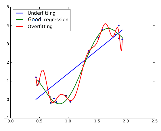
A regression problem is meant to provide an estimate of a function $y = f(x)$ on a given domain. If there is noise in the training dataset, it should not be taken into account by the model because it does not correspond to the true values of the function. In this figure, the red curve illustrates the overfitting phenomenon. Too much importance is given to the training error minimization without considering generalization.
Inversely, the blue curve does not enough take the training error into account, which also provides bad approximation results. The green curve, on the other hand, shows an example of good balance between training error minimization and generalization.
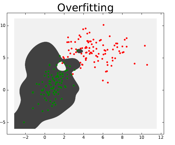
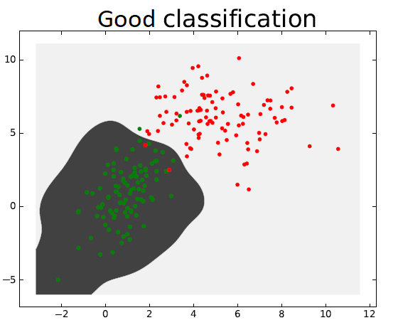
Classification example
In the classification case, a model is said to overfit a dataset when it classifies correctly each of its training instances, including the outliers. The following left figure illustrates well this issue.
Cross Validation
In order to check if a given Machine Learning model generalizes well to new data, we use a method called cross validation. Such method enables, among other things, to check that there is no overfitting.
-
The first very basic idea that comes to mind in order to test if a trained model is good for inference is called resubstitution. It consists in passing the training data through the classification model and compare the classes predicted with their true target values. Generally speaking, such method is a bad idea. Indeed, the points used for such validation method have already been used to train the model and if the model has overfitted these points, $100\%$ of the predictions should be correct. However, such a good validation result would not mean that the model generalizes well to other points.
-
The three (similar) validation methods explained in the following sections all start with a randomization of the dataset. Such procedure enables to throw off any possible correlation between nearby data points and to increase the probability to select a subset that is representative of the real data.
-
Once the dataset have been mixed up, the first validation method presented (called hold out) consists in splitting the data into two subsets, one for training the model (the training set) and one for its validation (the validation set). Once the initial dataset has been split, the model is trained using only the training set. Then we can check that the model is good at inferring new data by comparing the targets and the predictions on the validation set. If the validation error is low, we can assert with better confidence that the model is reliable and able to generalize to new data. Generally speaking, we use $60$ to $80\%$ of the data for training and the rest for validation.
-
The $K$-fold validation method is an extension of the Hold-out method. The idea is to split the initial dataset (after randomization) into $K$ subsets of equal size. Then a Hold-out validation is carried out, using $K-1$ subsets for training and $1$ for validation. This process is repeated $K$ times, so that each group is used for validation once. The validation error is then the mean of all the Hold-out errors obtained. By using this technique instead of the Hold-out method, the risk of an unfortunate bad choice of the validation set during sampling is decreased.
-
Finally, the last validation method is an extension of the K-fold method. It is called the Leave-one-out method and it is simply a $K$-fold validation where $K = N$, with $N$ the total number of available training data. In other words, we leave one data point out of the training set, train the model and check if it predicts the class of the point well. This process is repeated $N$ times.
The methods presented above are used to validate the choice of a certain model and the hyperparameters of the algorithm. Generally speaking, if a learning model was well designed, the more data it uses, the better its predictions are. Hence, once a model has been validated by one of the methods above, it is smarter to retrain the classification model with all the data available before using it to classify new unlabelled data.
Exercise[$K$-fold validation for $K$-nearest neighbors]
-
Implement the $3$-fold validation method on the Iris dataset, for the $3$-nearest neighbors algorithm.
Algorithms require to choose a certain number of parameters before training the model on the example labelled data. Such parameters are called hyperparameters. For instance, with the K-nearest neighbors algorithm, the user needs to select the value of the integer $k$, the number of neighbors to take into account for predicting the class of a feature vector. Usually, the choice of the hyperparameters greatly influence the quality of the obtained classifier. In order to choose such parameters properly, we will use a method similar to the methods used for model validation. The underlying idea is to split the example dataset into three parts, one for training $(\sim80\%)$, one for testing the parameters $(\sim20\%)$ and one for validation of the chosen model $(\sim20\%)$. Then, several models are trained on the training set (using different values of the hyperparameters) and compared using the testing set. The set of hyperparameters with lowest testing errors is selected and the model obtained is validated using the validation set. This way of proceeding avoids the unfortunate possibility of selecting hyperparameters that fit specifically the testing set. Indeed if it works well on the validation set (which had no influence on the hyperparameters selection), it is likely to be a good model.
Exercise[Parameter selection on $K$-nearest neighbors]
-
Implement the parameters selection method presented above in order to choose a good $k$ for the Iris dataset classified with the $K$-nearest neighbors algorithm.
Perceptron
What is a neural network? To get started, I'll explain a type of artificial neuron called a perceptron. Perceptrons were developed in the 1950s and 1960s by the scientist Frank Rosenblatt, inspired by earlier work by Warren McCulloch and Walter Pitts. Today, it's more common to use other models of artificial neurons. So how do perceptrons work? A perceptron takes several binary inputs and produces a single binary output.
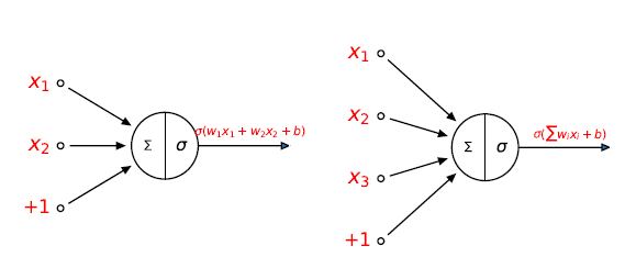
In this example, the perceptron has two inputs, $x_1$ and $x_2$. Function $\sigma $ is an activation function. The output of the second perceptron neuron is given by $\sigma \left(w_{1}x_{1}+w_{2}x_{2}+w_{3}x_{3}+bx_{4}\right)$ where the input $x_{4}$ is always equal to $1$. In general it could have more or fewer inputs. Rosenblatt proposed a simple rule to compute the output. He introduced weights, $w_1,w_2,…,$ real numbers expressing the importance of the respective inputs to the output. The neuron's output, $0$ or $1$, is determined by whether the weighted is less than or greater than some threshold value $b$. Just like the weights, the threshold is a real number which is a parameter of the neuron. To put it in more precise algebraic terms:
- $output = \sigma \left( w_{1}x_{1}+w_{2}x_{2}+\cdots +w_{n}x_{n}+b\right)$ where $\sigma \left( x\right) =\left \{ \begin{array}{rl} +1 & \text{if }x\geqslant 0 \\ 0 & \text{else} \end{array} \right. $
- $w_{1}x_{1}+w_{2}x_{2}+\cdots +w_{n}x_{n}+b=0$ defines an hyperplane which divides the input space into two parts
- The perceptron is used to decide whether an input vector belongs to one of the classes, say classes A ($+1$) and B ($0$)
Let us define the code of the perceptron algorithm for the logical OR function. The perceptron algorithm needs to map the possible input to the expected output. The first two entries of the NumPy array in each tuple are the two input values. The second element of the tuple is the expected result. And the third entry of the array is a "dummy" input (also called the bias) which is needed to move the threshold (also known as the decision boundary) up or down as needed by the step function. Its value is always $1$, so that its influence on the result can be controlled by its weight. Next we'll choose three random numbers between $0$ and $1$ as the initial weights. In order to find the ideal values for the weights w, we try to reduce the error magnitude to zero. In this simple case $n = 50$ iterations are enough; for a bigger and possibly "noisier" set of input data much larger numbers should be used. First we get a random input set from the training data. Then we calculate the dot product (sometimes also called scalar product or inner product) of the input and weight vectors. This is our scalar result, which we can compare to the expected value. If the expected value is bigger, we need to increase the weights, if it's smaller, we need to decrease them. This correction factor is calculated in the last line, where the error is multiplied with the learning rate $eta$ and the input vector $x$. It is then added to the weights vector, in order to improve the results in the next iteration.
from random import choice
from numpy import array, dot, random

def sigma(x):
    if x<0:
        return 0.0
    else:
        return 1.0

training_data = [
            (array([0,0,1]), 0),
            (array([0,1,1]), 1),
            (array([1,0,1]), 1),
            (array([1,1,1]), 1),
            ]
w = random.rand(3)
errors = []
eta    = 0.5
n      = 50
# Learning step
for i in range(n):
    x, expected = choice(training_data)
    result = dot(w, x)
    error = expected - sigma(result)
    errors.append(error)
    w += eta * error * x

# Prediction step
for x, _ in training_data:
    result = dot(x, w)
    print("{}: {} -> {}".format(x[:2], result, sigma(result)))
Exercise[Other logical functions]
- Change the training sequence in order to model an AND, NOR or NOT function.
- Is it possible to model the XOR function?
- Adapt the previous algorithm to the 2D following generated data.
- Give according to the $eta$ parameter the convergence speed
- Draw in the same graphic the evolution of the hyperplane and the data
import numpy as np
from numpy import array, dot, random
import matplotlib.pyplot as plt

# Learning step
p = 150
R = 1.5
t = np.linspace(0, 2*np.pi, p)

# First class +1
x1= [ 1+R*random.rand()*np.cos(t[n]) for n in range(p) ]
y1= [ 1+R*random.rand()*np.sin(t[n]) for n in range(p) ]

# Second class 0
x2= [ -1+R*random.rand()*np.cos(t[n]) for n in range(p) ]
y2= [ -1+R*random.rand()*np.sin(t[n]) for n in range(p) ]

plt.scatter(x1,y1,c='red', marker = 'o', s=4)
plt.scatter(x2,y2,c='green', marker = 'o', s=4)
plt.title('Perceptron algorithm')
plt.savefig('datapoints.png')
plt.show()
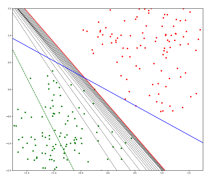
The main objective is to split the data points into two different sets with a linear segment. As we can see, there exists an infinite number of solutions.
Support Vector Machine (SVM)
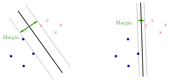
This algorithm will only be studied in its linear form in this class. The SVM algorithm consists in finding the hyperplane such that the margin between the two parallel hyperplanes on both sides that fully separates the training set is maximized. As illustrated on the following figure in the two dimensional case. On this figure, both black lines correctly separate the dataset but the one on the left is a better classifier as the margin is wider. Intuitively, the model on the left appears to generalize better than the one on the right.
When the two classes are not linearly separable, certain points are allowed to enter the margin (soft margin). The notion of error is introduced, it is written $\epsilon$ and defined as showed on this figure.
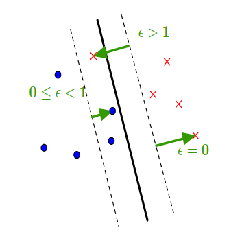 We note that the error associated to a point correctly classified and outside the margin is zero.
Then, the goal is to find the line (hyperplane) that maximizes the margin while minimizing the errors. In other words, we want to minimize the following function:
\begin{equation}
\label{eq:minimization_svm}
\begin{aligned}
& \underset{dataset}{\text{Minimize}}
& & \frac{1}{margin} + C \times \sum_i\epsilon_i \\
\end{aligned}
\end{equation}
Hence, to create a good SVM model, the first step is to select a good value for the parameter C. The bigger C is, the more we want to minimize the training error. Likewise, a small C means that emphasis is put on maximizing the margin.
A large margin corresponds to good generalization, and the art behind designing a good SVM algorithm is to find the right value of C, balancing between overfitting (margin too small, C too large) and underfitting (margin too large, C too small).
We note that the error associated to a point correctly classified and outside the margin is zero.
Then, the goal is to find the line (hyperplane) that maximizes the margin while minimizing the errors. In other words, we want to minimize the following function:
\begin{equation}
\label{eq:minimization_svm}
\begin{aligned}
& \underset{dataset}{\text{Minimize}}
& & \frac{1}{margin} + C \times \sum_i\epsilon_i \\
\end{aligned}
\end{equation}
Hence, to create a good SVM model, the first step is to select a good value for the parameter C. The bigger C is, the more we want to minimize the training error. Likewise, a small C means that emphasis is put on maximizing the margin.
A large margin corresponds to good generalization, and the art behind designing a good SVM algorithm is to find the right value of C, balancing between overfitting (margin too small, C too large) and underfitting (margin too large, C too small).
Multiclass classification
As for all classification models using separating hyperplanes, SVM can only classify elements belonging to two different classes because a hyperplane separates the space in only two distinct subspaces. For a point $x^*$, if the separating hyperplane is in the form $$ d(x) = 0, $$ and if we note $C_i$ the class $i$, we can assert that \begin{array}{cccc} & x^* \in C_1 & \text{if} & d(x^*) \geq 0 \\ \text{and} & x^* \in C_2 & \text{if} & d(x^*) \leq 0. \end{array} When there are more than two classes (e.g. Iris), there exist two possible approaches.
One vs Rest
For each class $C_i$, we create a hyperplane that separates $C_i$ from all other classes. We call $d_i$ such a separating hyperplane and we have the following condition for a point to be a member of class $C_i$:
$$
x* \in C_i \Leftrightarrow
\left\{\begin{array}{l} d_i(x^*) > 0 \\ d_j(x^*) < 0 \; \forall j \neq i \end{array}\right.
$$
The following figure shows the different hyperplanes as well as the classification zones they define. This exemple represents a bidimensional case with three classes.
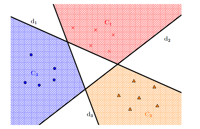 The white areas represent points which does not belong to any class. A more permissive way to define the class membership of a point is by choosing $C_i$ that goes with the largest $d_i(x)$.
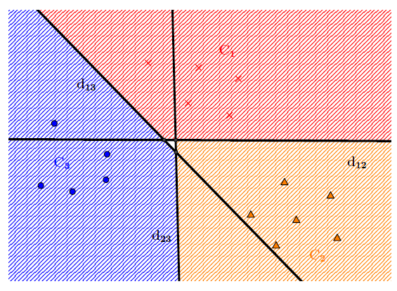
For each pair $\{i,j\}$, a hyperplane separating $C_i$ from $C_j$ is computed and noted $d_{ij}$. Then, we have the following condition for the membership of a new point:
$$
x* \in C_i \Leftrightarrow
\left\{\begin{array}{l} d_{ij}(x^*) > 0 \; \forall i \neq j \\ d_{ij}(x^*) = - d_{ji}(x^*) \; \forall j \neq i \end{array}\right.
$$
- Implement multiclass linear SVM for the Iris dataset.
- Run a parameter selection procedure and a cross validation to determine the best value for parameter $C$.
References
- Franck Rosenblatt (1962), Principles of neurodynamics: perceptrons and the theory of brain mechanisms