Neural Network

Introduction

The concept of neural network is explored through the most classical architecture : The multi-layer perceptron (MLP). Many other neural network architectures exist in the literature but they all share some of the basic principles defined here. The more basic element of a neural network is called a neuron. It is defined by the following diagram. 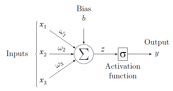Given an input vector $x$, of dimension $n$ ($3$ on the figure), a neuron is defined by $n$ weights $\{\omega_1, \ldots, \omega_n\}$, a bias $b$ and an activation function $\sigma$. The idea is that the activation function should receive an affine combination of the entries: $z = \sum_i (\omega_i x_i) + b$. Thus, for a given input $x$, the output $y$ of the neuron is defined by $$ y = \sigma(\sum_i (\omega_i x_i) + b). $$ A few commonly used activation functions $\sigma$ are:

• the logistic function : $y = \frac{1}{1+e^{-z}}$
• the hyperbolic tangent function : $y = tanh(z)$
• the RELU (REctified Linear Unit) : $y = max(0, z)$

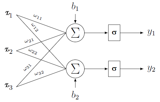
After defining what a neuron is, we can introduce the notion of layers of neurons. We call layer a group of neurons sharing the same inputs. Each neuron has its own weights and bias but is left-connected to the same input vector than the other neurons in the layer. One layer has as many outputs as its number of neurons. Thus, on the following figure, we can see a layer with two neurons (and two outputs) and a three dimensional input vector.

Multi-layer perceptron (MLP)

A multi-layer perceptron is a stacking of several layers. The outputs of one layer are the inputs of the next layer. Hence, to carry out a regression with $M$ outputs, the last layer should be composed of $M$ neurons. As the dimension of the last layer is fully determined by the data, we call hidden layers all the other layers of the network. The following figure shows a diagram representing a MLP with three inputs, two outputs and one hidden layer with three neurons. 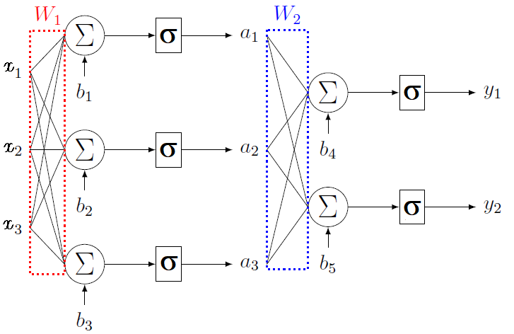This MLP has three inputs, one hidden layer and two outputs.

Neural networks are called universal approximators, which means that it is possible to approximate any function on a closed and bounded space in $\mathbb{R}^n$ by a neural network with only one layer. Such neural network architecture can reach any given precision. The universal approximation theorem is formalized as follows.

Training a Neural Network

As for all other models we have seen so far, training a neural network consists in finding a set of parameters minimizing the errors on the training set and enabling good generalization. For a neural network, the parameters that can be tuned are the weights and the biases of each neuron. The principle behind the optimization of these weights is based on gradient descent. Gradient descent is an optimization technique that modifies the weights iteratively for each training data, according to the observed error, as shown on the following figure. 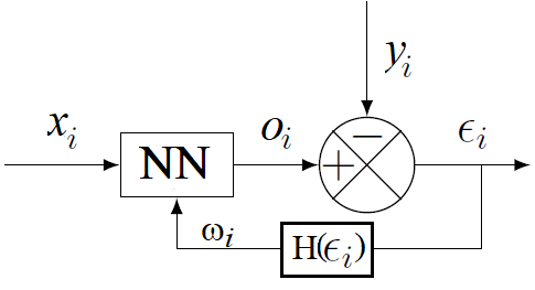Let us given the input values $x_i$ then we compare the output $o_i$ of the neural network with the "true" value $y_i$. According to the error values $\epsilon_i$ the weights of the neural networks are modified according to a gradient algorithm, denoted by $H$, such that we minimize a given loss function.

Exercise[Tune the parameters of a MLP]

• Implement a neural network using scikit-learn library to approximate the function $$f(x) = x^2 + sin(5x)$$ between $0$ and $\pi$. We will use synthetic data.

        
import numpy as np
import sklearn.neural_network as nn

# Function to approximate
def f(x):
    return x**2 + np.sin(5*x)

# Synthetic dataset generation
inf_bound = 0
sup_bound = np.pi
N_train = 100
N_test = 20
X = np.array([[np.random.uniform(inf_bound, sup_bound)] for i in range(N_train)])
Y = np.array([f(x) for x in X])

# Neural Network Learning process
model = nn.MLPRegressor(hidden_layer_sizes = (10, 10, 10, 10), activation = 'tanh', solver = 'lbfgs',  max_iter = 100000)
model.fit(X, Y)
# Neural network data test set
X_test = np.array([[np.random.uniform(inf_bound, sup_bound)] for i in range(N_test)])
Y_test = np.array([f(x) for x in X_test])
# Neural network prediction
Y_pred = model.predict(X_test) 
Y_pred = np.reshape(Y_pred,(N_test,1)) 
# Errors between the model and the True values
errors = np.abs(Y_test - Y_pred)

print('Mean test error :', np.mean(errors[:, 0]))
print('Max test error  :', np.max(errors[:, 0]))

        
    

As we can see we use four hidden layers for the Neural Network model and the $\mathbf{\tanh}$ function as an activation function. The lbfgs algorithm is used in order to minimize the least square function of the differences between the true values of $Y$ and the predicted values of the model at each iteration of the algorithm.

• Same question for $f(x) = [x_0^3 \times sin(2 \times x_1)^2, x_2^2+x_0]^T$. By modifying the parameters of the neural network model, compute the errors.

• Derive the direct model linking angular positions to Cartesian position of a 2D planar robot with two axes (each of length $2$).

• Use this model to generate training data for the inverse model.

• Train a neural network to estimate the inverse model.

If needed, you can limit the validity of the inverse model to a certain range of Cartesian points and the outputs to a certain range of angular values.

References

- Franck Rosenblatt (1962), Principles of neurodynamics: perceptrons and the theory of brain mechanisms
- Xavier Glorot and Yoshua Bengio (2010), Understanding the difficulty of training deep feedforward neural networks. In Proceedings of the International Conference on Artificial Intelligence and Statistics (AISTATS’10). Society for Artificial Intelligence and Statistics.