Unsupervised Classification

Introduction

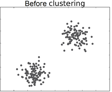
Unsupervised classification (also called clustering) is the problem of classifying a dataset without any labels for training. An unsupervised learning algorithm is supposed to find tendencies, similarities between certain feature vectors. The goal is to group data within clusters, such that the members of one cluster are as similar as possible while being as different as possible from other clusters members.

The following video shows an application of clustering to unsupervised sorting of objects by a robotics system.

K-means Algorithm

The K-means clustering algorithm principle is the following. Starting from a given dataset, the space is partitioned by centroids in the $N$ dimensional space. These centroids are simply points in this space. A data point belongs to the class represented by the centroid that is closest to itself according to the norm used (usually the euclidean norm). Hence, there should be as many centroids as the number of desired classes. The successive steps executed by $K$-means are the following.

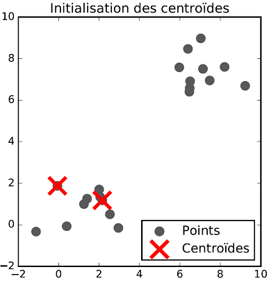
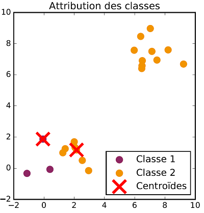
• Centroids initialization: The $K$-means algorithm works in an iterative fashion. The first step consists in initializing the centroids. If we want to classify the data within $K$ classes, then $K$ points (with the same dimension as the feature vectors) must be introduced. There exist different methods to position such points, one of them is to choose $K$ random points among the dataset and to let the initial centroids be these points.

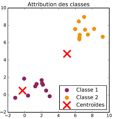
• Classes allocation: Once centroids are defined, the next step is to label each point according to the current centroids. Hence, for each point, we must compute its distance to each centroid and label it with the class corresponding to the closest one.

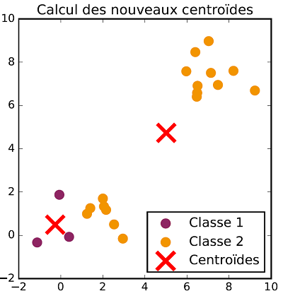
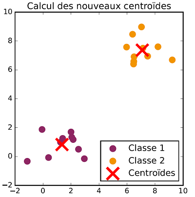
• Centroids updating: Once every point in the dataset has got a label, centroids are updated. For each one of the current classes, the mean vector is computed and the new value of the class centroid is set equal to this mean vector.

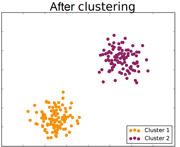
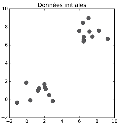
The class allocation and centroid update steps are repeated successively until there is no more evolution in both steps. Once the process is over, data are classified. The following figures show the different steps of $K$-means clustering on a two dimensional dataset with two classes.

Exercise[$K$-means clustering implementation]

• Implement the $K$-means clustering algorithm on the Iris dataset without using the labels (Labels can be used to check the clustering results).

• Do the same thing with the "Wine" dataset, which can be found at this link

We want to segment a color image (Red, Green, Blue) by applying the k-means algorithm.


In this example, we segmented the original image with $K = 3$ classes. You can download the Nao image by using the following link NAO

• For this, we create a data set of 3d points issued from the color map of the original image. The matplotlib library is used to manipulate the image. For instance, the following code:

  import matplotlib.pyplot as plt
  import matplotlib.image as mpimg
  import numpy as np
  img = mpimg.imread(”peppers.png”)
  
  plt.imshow(img) # print the image
  plt.show()
  print(img[100,120,0]) # print the red pixel value for row 100 and column 120
  print(img[100,120,1]) # print the green pixel value for row 100 and column 120
  print(img[100,120,2]) # print the blue pixel value for row 100 and column 120
  print(img.shape) # print the dimensions of the image
  
                      

  allows us to set the image in a numpy array. We can create a 400x600 color image by using:

  image=np.zeros((400,600,3),dtype=np.float32)
                      

  Or create a gray level 400x600 image with:

  image=np.zeros((400,600),dtype=np.float32)
                      

  or copy an image:

  im=np.copy(image)
                      

• Let us given $k$, the number of class segmentation. By applying the k-means algorithm defined a Target list where for each index of the list you calculate the associated class segmentation value: $0,1,2,...,k-1$. Then, define a function which returns a gray level image where for each pixel of the image is associated the class segmentation value. Draw this image.

• Show for some examples that the segmentation result is sensitive or not to the initial centroids. You can also modify the value of $k$.

    from random import uniform
    import numpy as np
    import matplotlib.pyplot as plt
    from numpy import linalg as LA
    import matplotlib.image as mpimg
    
    def distance(P,Q):
        Q=np.dot(-1,Q)
        R=np.add(P,Q)
        return LA.norm(R,2)
    
    def get_classes(P,Q):
        n=len(P)
        target=np.zeros(n)
        # TO DO
        return target
    
    def update(P,target,K):
        n=len(P)
        c=np.zeros((K,3))
        p=np.zeros(K)
        # update the centroids 
        for i in range(n):
            # TO DO

        return q
    
    def split(img,Q,K):
        n,p,_ = img.shape
        res=np.zeros((n,p),dtype=np.float32)
        # TO DO
        return res       
        
    def segment(img,K, itermax = 30, eps = 0.001):
        n,p,_ = img.shape
        print(" dim = ",n," ",p)
        # TO DO
        return Q
    
    # Load a color image
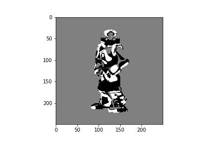
    im1 = mpimg.imread("nao2.png")
    plt.imshow(im1)
    plt.show()

    K = 3
    centroides=segment(im1,K)
    # print(centroides)
    im2=np.asarray(split(im1,centroides,K), dtype=np.float32)
    plt.gray()
    plt.imshow(im2)
    plt.savefig('nao_seg.png')
    plt.show()

References

- Franck Rosenblatt (1962), Principles of neurodynamics: perceptrons and the theory of brain mechanisms