Simulated Annealing Algorithm
Simulated Annealing with Constraints
The objective is to implement the simulated annealing algorithm. Indeed, for complete NP optimization problems, such as the problem of traveling salesman, we don't know a polynomial algorithm allowing an optimal resolution. We will therefore seek an approximate solution of this optimum using heuristics. Simulated annealing is an algorithm based on a heuristic allowing the search for a solution to a problem given. It allows in particular to avoid the local minima but requires an adjustment of its parameters. The simulated annealing algorithm can be represented as follows:
            We set an initial vector configuration X
            Xopt = X
            Set an intial Temperature
            While (Temperature > Final Temperature and nbiter< itermax) do
            {
                Repetition=1
                while (Repetition <= MaxTconst) do
                {
                    Randomly choose Y in the vicinity of vector X
                    DJ = J(Y ) - J(X)
                    if DJ < 0 then
                    {
                        X = Y
                        if J(X) < J(Xopt) then
                            Xopt = X
                    }
                    else
                    {
                    Choose randomly p in [0, 1]
                    if p <= exp(-DJ / T )
                        X = Y
                    Repetition = Repetition + 1
                    }
                }
                nbiter=nbiter+1
                T = g(T)
            }
            return Xopt
This algorithm have different parameters:
- The Initial Temperature: Tinit
- The Final Temperature: Tf
- The function g that enables the decrease of the temperature at each step of the algorithm
- The amplitude of the random choose in the vicinity of the current value of the state: Ampli
- The number of iterations at the same temperature: MaxTconst
At the beginning, the initial temperature is high so even if we choose a random value $Y$ in the vicinity of the current $X$ such that $J(Y)>J(X)$ we will accept this "increase" of $J$ even if we search for a minimum. This methodology avoids to "fall" in a "bad" local minimum. The probability of this increasing is very high at the beginning and it decreases a lot as soon as the temperature decreases. We allow this increase step by comparing the random value $p$ to this value $e^\frac{-DJ}{T}$. If $T$ is high this value is very close to $1$. As soon as $T$ decreases the value of this exponential tends to zero. Consequently, the probability that $p$ even choosen randomly be less than this value becomes very low during the iteration process.
Exercise [Simulated Annealing with one variable]-
Implement this algorithm in the following function:
def Recuit(Xinit, Tinit, Tf, Ampli, MaxTconst, itermax). This function returns a list: $Xopt$ and all the iterative values of $X$. We assume that function $g(T)$ is equal to $T^{0.99}$. This allows that the temperature decreases slowly. -
Apply this algorithm with the following functions:
def J(X): return (X[0]**2-4*X[0]+4)*(X[0]**2+4*X[0]+2) + X[1]**2 def g(T): return T**0.99 -
Tune the parameters such that you obtain the global minimum $(-1-\sqrt{2},0)$.
        def Recuit(Xinit, Tinit, Tf, Ampli, MaxTconst, itermax):
            j=1
            X = Xinit
            T = Tinit
            L =[X]
            Xopt = X
            while(T > Tf and j < itermax):
                compteur = 1
                while(compteur <= MaxTconst):
                    Y=[]
                    for i in range(len(X)):
                        s=X[i]+Ampli*(-1.0+2.0*np.random.random_sample())
                        Y.append(s)
                    DJ=J(Y)-J(X)
                    if(DJ < 0.0):
                        X = Y
                        L.append(X)
                        if(J(X) < J(Xopt)):
                            Xopt = X
                    else:
                        p = np.random.random_sample()
                        if(p <= np.exp(-DJ/T)):
                            X = Y
                            L.append(X)
                    compteur = compteur + 1
                T = g(T)
                j = j + 1
            return [Xopt, L]

        res,x=Recuit([1],1000.0,1.0,0.5,2,100)
        print(x)
        print("xopt= ",res," true value= ",-1-np.sqrt(2))
Exercise [Simulated Annealing with two variables and constraints]
-
Implement this algorithm for the following function:
def J(X): return X[0]**2+X[1]**2 -
We wish to apply this algorithm to the following constraint problem: $$ \min\limits_{(x_0,x_1) \in \mathbb{R}^{2}} J(x_0,x_1)=x_0^2+x_1^2 $$ such that $$ g_1(x_0,x_1) = (x_0-2)^2+x_1^2-1=0 $$ Optimizing this problem with this algorithm is almost impossible because satisfying the constraint of $g$ at each step by choosing the variables $x_1$ and $x_2$ randomly such that $g_1(x_0,x_1)=0$ is impossible. It's why we modify the equality constraint $g_1(x_0, x_1) = 0$ under the form of two inequalities in order to release this constraint:
$g_1(x_0, x_1)-\epsilon \leq 0$ and $-g_1(x_0, x_1)-\epsilon \leq 0$.
where parameter $\epsilon$ is a small value to be defined. This method also requires that the initial values verify the inequality constraints from the start. Write the Annealing function RecuitC which takes into account the inequality constraints.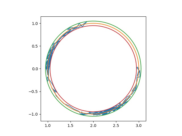
        def J(X):
            return X[0]**2+X[1]**2

        def Recuit(Xinit, Tinit, Tf, Ampli, MaxTconst, itermax):
            j=1
            X = Xinit
            T = Tinit
            L =[X]
            Xopt = X
            while(T > Tf and j < itermax):
                compteur = 1
                while(compteur <= MaxTconst):
                    Y=[]
                    for i in range(len(X)):
                        s=X[i]+Ampli*(-1.0+2.0*np.random.random_sample())
                        Y.append(s)
                    DJ=J(Y)-J(X)
                    if(DJ < 0.0):
                        X = Y
                        L.append(X)
                        if(J(X) < J(Xopt)):
                            Xopt = X
                    else:
                        p = np.random.random_sample()
                        if(p <= np.exp(-DJ/T)):
                            X = Y
                            L.append(X)
                    compteur = compteur + 1
                T = g(T)
                j = j + 1
            return [Xopt, L]

        res,X=Recuit([1,2],1000.0,1.0,0.5,2,200)
        print("xopt= ",res)
        eps=0.1
        def G(X):
            return [(X[0]-2)**2+X[1]**2-1-eps,-(X[0]-2)**2-X[1]**2+1-eps]

        def RecuitC(Xinit, Tinit, Tf, Ampli, MaxTconst, itermax):
            j=1
            X = Xinit
            T = Tinit
            L =[X]
            Xopt = X
            while(T > Tf and j < itermax):
                compteur = 1
                while(compteur <= MaxTconst):
                    Y=[]
                    for i in range(len(X)):
                        s=X[i]+Ampli*(-1.0+2.0*np.random.random_sample())
                        Y.append(s)

                    # Test if the Y vector satisfies all the constraints
                    # if not we choose an another value

                    if G(Y)[0] <=0 and G(Y)[1] <=0: # if G has more two constraints adapt the code
                        DJ=J(Y)-J(X)
                        if(DJ < 0.0):
                            X = Y
                            L.append(X)
                            if (J(X) < J(Xopt)):
                                Xopt = X
                        else:
                            p = np.random.random_sample()
                            if(p <= np.exp(-DJ / T)):
                                X = Y
                                L.append(X)
                    compteur = compteur + 1
                T = g(T)
                j = j + 1
            return [Xopt, L]
        # We choose an initial value which satisfies the constraint functions
        Xinit = [3,0]
        res=RecuitC(Xinit,1000.0,1.0,0.2,2,1500)
        print(res[0])
Exercise [Simulated Annealing for beam problem]
We want to determine the optimal section $(b, h)$ of a beam (poutre encastrée) of length $L = 1000mm$ and subject to a force $F = 1000N$. By using the RecuitC function find a solution to this constraint problem: $$ \min\limits_{(b,h) \in \mathbb{R}^{2}} J(b,h)=bhL $$ such that
- $fleche_{maxi}(b,h) \leq 2.5$mm
- $\sigma_{max}(b,h) \leq \sigma_{acier}$
- $6 \leq \dfrac{h}{b} \leq 25$
- $-h \leq 0 \text{ and } -b \leq 0$
-
Find an optimal solution to this beam problem
Exercise [Simulated Annealing for transport problem]
Le problème de transport se présente de la manière suivante : on désire acheminer des marchandises de $n$ dépôts à $m$ points de ventes, connaissant $c_{i,j}$ pour $i = 1,...n$ et $j= 1,... ,m$ les coûts de transport entre tous les couples $(i, j)$. Les valeurs $Q_i$ pour $i =1,...,n$ sont les quantités produites et disponibles au dépôt $i$. Les quantités entières $D_j$ pour $j=1,..., m$ sont les niveaux de demande aux points de vente (ou client) $j$. On fera l’hypothèse que les $c_{i,j}$ correspondent au nombre de kilomètres entre les points de production $i$ et les clients $j$. On recherche pour chaque couple $(i, i)$ la quantité (positive) $x_{i,j}$ transportée du dépôt $i$ au point de vente $j$, c-à-d la solution du problème linéaire
$$ \min_{x_{i,j} \geq 0} \sum_{i=1}^{n}\sum_{j=1}^{m} {c_{i,j}x_{i,j}} $$ sous les contraintes $\displaystyle{\sum_{i=1}^{n}}x_{i,j} = D_j,(j= 1,...,m) $ et $\displaystyle{\sum_{j=1}^{m}}x_{i,j} = Q_i, (i = 1,... ,n)$Le critère représente le coût total de transport. Les contraintes expriment l'égalité de l'offre et de la demande pour chaque point de vente et chaque dépôt. On peut relaxer la contrainte on supposant que l’on souhaite au plus satisfaire la demande. Les contraintes de type égalité sont aussi transformées en contraintes inégalité si $\displaystyle{\sum_{i=1}^{n}} Q_i \geq \displaystyle{\sum_{j=1}^{m}} D_j$
- Tirer au hasard les points de production et les points associés aux clients. Tracer ces points puis calculer les distances $c_{i,j}$ entre les points $i$ et $j$. Tirer au hasard les quantités produites $Q_{i}$ de l'entrepôt $i$ ainsi que les valeurs des demandes $D_j$ de chaque client $j$. On supposera que ces valeurs sont des entiers positifs.
- Ecrire le problème d'optimisation avec inégalités
- Intialiser les $x_{ij}$ en utilisant la méthode dite du coin Nord-Ouest
- Résoudre ce problème avec le Recuit simulé sous contraintes
- Tracer la solution ainsi obtenue
Simulated Annealing and shortest path
In this Section, we adress the problem of finding the shortest paths between nodes in a graph,
which may represent, for example, road networks. For example, if the nodes of the graph represent cities
and edge path costs represent driving distances between pairs of cities connected by a direct road
(for simplicity, ignore red lights, stop signs, toll roads and other obstructions),
we want to define algorithms that can be used to find the shortest route between one city and all other cities.
A widely used application of shortest path algorithm is network routing protocols.
Let $P$ be $n+1$ a set of data point. $P$ being a list.
We wish to find the shortest path between points. For this, we need to calculate the distance between each data point. The so calculated path, interpolates one time maximum each data point.
We then wish to calculate the shortest path making it possible to pass at most once by all the points of $P$.
Consequently, a given sequence of points is bijectively associated with a circular permutation:
$\sigma$ of
$\left\{ 0,\ldots,n\right\}$.
For example the following permutation:
$$
\left(\begin{array}{ccccc}
0 & 1 & 2 & 3 & 4\\
1 & 4 & 3 & 2 & 0
\end{array}\right)
$$
gives $\sigma\left(0\right)=1$, $\sigma\left(1\right)=4$, $\sigma\left(2\right)=3$, $\sigma\left(3\right)=2$ and $\sigma\left(4\right)=0$.
We denote by $E$ the function which gives to a given permutation $\sigma$ the total length:
$$
E\left(\sigma\right)=\sum_{i=0}^{n}\parallel P_{\sigma\left(i+1\right)}-P_{\sigma\left(i\right)}\parallel
$$
where the condition
$$
\sigma\left(n+1\right)=\sigma\left(0\right)
$$
allows to close the path. The value $E\left(\sigma\right)$ is then the total length of the path.
Therefore, we have to find the permutation which minimizes $E$. This optimization problem involves the set of permutations of $n+1$ elements. Evaluating $E$ on all permutations takes a very long time even for a not too large $n$. This problem is more complicated than it seems; there is no known method of resolution making it possible to obtain exact solutions in a reasonable time. We must therefore approximate the solution, because we are faced with a combinatorial explosion.
For a set of $n+1$ points, there are $(n + 1)!$ possible paths. The starting point does not change the length of the path, we can choose it arbitrarily, so we have $n!$ different paths. Finally, each path can be traveled in two directions and the two possibilities having the same length, we can divide this number by two. So we have $\frac{n!}{2}$ possible paths.
For example, with $n=71$ data points, the possible number of paths is around $6.10^{99}$. No comment !
We therefore use a probabilistic algorithm called simulated annealing which will make it possible to answer the question in an approximate manner in a much shorter time even for large values of $n$.
To build this algorithm, we imagine that the function to be optimized is the energy of a fictitious physical system. At initialization, our physical system has an energy $E_{0}$ and is brought to a temperature $T_{0}$.
We assume that the state associated with the initial energy $E_{0}$ is $X_{0}$. The temperature is a parameter of the algorithm. Then we apply the laws of statistical physics to our fictitious physical system. The energy state of our physical system fluctuates around an average energy which is linked to the temperature. This means that the variable $X$ belongs to an interval $[X−δX,X+δX]$ where $δX$ is a random vector. Once equilibrium has been reached, the temperature is slightly reduced and the search for thermal equilibrium is started again with the new temperature. The temperature is thus reduced until a low limit temperature is reached, which is another parameter of the algorithm. We assume that the system reaches the minimum energy state of the fictitious physical system.
How to determine the random fluctuations of the energy of our system?
Statistical physics tells us that the probability of finding a system in an energy state $s$ is proportional to $e^{-\frac{E_{s}}{T}}$. The Metropolis algorithm that we are going to use proposes a method of random fluctuation based on this law:
Let $X_{i} $ be an energy state $E_ {i}$, then by adding a random quantity to it we then pass to the state $X_{i + 1}$ which corresponds to an energy $E_{i+1}$. If $E_{i+1} < E_{i}$ then $X_{i + 1}$ becomes the new state of the system, because its energy decreases.
Otherwise, we leave the system in the state $X_{i}$ or we make it evolve anyway to $X_{i + 1}$, which then becomes the new state of equilibrium, according to an equal probability at
$$
e^{-\frac{E_{i+1}-E_{i}}{k_{B}T}}
$$
There are however many parameters in this algorithm. In particular, the initial "temperature" of the system and its law of decay must be chosen. The initial "temperature" should be chosen high enough for thermal equilibrium to be reached quickly. This means that it must be large compared to the random variations of energy of the system. The decrease law of the temperature has been a tradeoff between the search for the best possible result and the calculation time.
We generally choose an exponential decay law of the type $T=T_{0} e^{-\frac{t}{\tau}}$ where $\tau$ is a large enough positive real value such that the decay is slow enough. The choice of the final temperature is also a tradeoff between the quality of the result and the calculation time. It depends on the nature of the problem to optimize. Here is the pseudocode of the simulated annealing algorithm applied to the optimization of a function $E(X_{1},...,X_{n})$.
-
Define the Energy function, the initial state $X$ of the system and the initial value $T_{0}$ of the temperature.
-
In the case of the shortest path, the function to optimize is the total distance to be traveled which is the sum of the distances between each of the pairs of neighboring points. The state of the system is characterized by the path between the different points and the associated total distance which is represented by its energy. To change the system state, we simply swap the order of some points in the $P$ list.
-
To minimize the energy $E$ we use the Metropolis algorithm (see below). The temperature is a control parameter with no particular functional significance. But the choice of the initial and final temperatures will constrain the efficiency of the algorithm.
-
Depending on the number of points, we will have a lot of calculations. It is therefore appropriate to optimize the code.
-
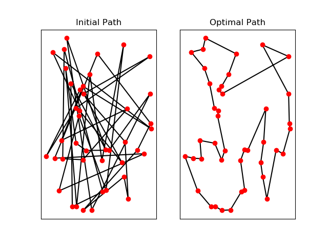
Generate the list of points where the coordinates of the points $(x,y)$ are drawn randomly according to the uniform law. The initial path is simply the indexing of the vector of the points according to their random coordinates initialized above. Save this initial path so that it can be displayed at the end of the calculation.
-
We choose $T0=10.0$, $Tmin=0.01$ and $tau=10000$.
The choice of the values of initial temperature and minimum temperature, that which fixes the end of the annealing, requires several tests. As a general rule, the value of $T0$ must be of the same order of magnitude as the energy variation.
The value of $ tau $ must be chosen large enough, so that the decrease in temperature is slow enough, but not too much so as not to have too many calculations. These parameters can be modified to study their influence on the results.
Exercise [Simulated Annealing for the salesman problem]
-
Define function Energy() which calculates the sum of the distances between the points in the order of the path.
-
Define the Fluctuation() function which swaps the points in the path between index $i$ and index $j$. This simulates an energy fluctuation in the system.
-
Implement the Metropolis algorithm:
""" The Metropolis function""" def Metropolis(E1,E2): global T,i,j # global variables if E1 <= E2: E2 = E1 # Energy of the new state else dE = E1-E2 if random.uniform() > exp(-dE/T): #The fluctuation is not accepted. #We then set the path in the previous state #by applying again the Fluctuation function Fluctuation(i,j) else: #The fluctuation is accepted E2 = E1 return E2 -
Code the main calculation loop of the simulated annealing algorithm. For this, you need to apply the Fluctuation(i,j) function where the indexes $i$ and $j$ are drawn as random variables. Consequently, this function creates a new path with a new Energy. Apply the Metropolis function so as to accept or not this new state path. Decrease the temperature according to the following law: $T = T0*exp(-t/tau)$
-
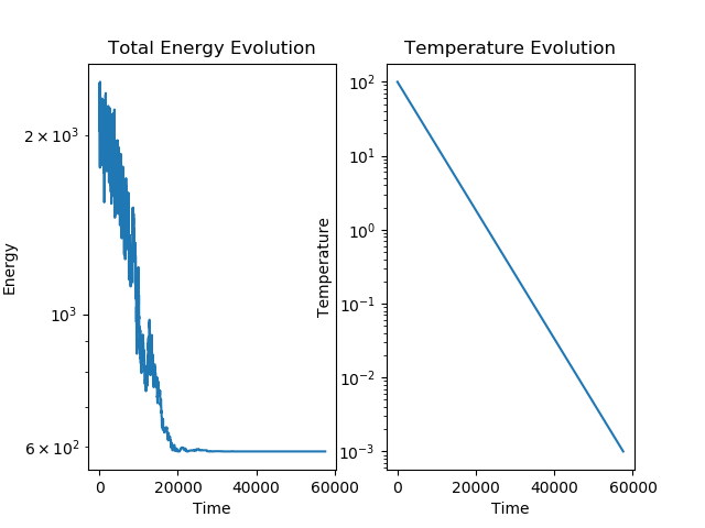
Draw the final path and the Energy history according to the temperature evolution. For this, you can use a logarithmic scale (see below).
import numpy as np
import matplotlib.pyplot as plt

""" The Energy function"""
def Energy():
    s = 0.0
    #TO DO
    return s

""" The Fluctuation function"""
def Fluctuation(i,j):
    #TO DO

""" The Metropolis function"""
def Metropolis(E1,E2):
    #TO DO
    return E2


# initialisation des listes d'historique
Henergie = []     # énergie
Htemps = []       # temps
HT = []           # température

N = 20 # number of cities or points
# paramètres de l'algorithme de recuit simulé
T0 = 100.0
Tmin = 1e-3
tau = 5000
x = random.uniform(size=N)
y = random.uniform(size=N)

# défintion du trajet initial : ordre croissant des villes
trajet = np.arange(N)
trajet_init = trajet.copy()

# calcul de l'énergie initiale du système (la distance initiale à minimiser)
Ec = Energy()

# boucle principale de l'algorithme de recuit simulé
t = 0
T = T0
while T > Tmin:
    # TO DO
    # historisation des données
    if t % 10 == 0:
        Henergie.append(Ec)
        Htemps.append(t)
        HT.append(T)

print("distance initiale= ",Henergie[0]," distance finale= ",Henergie[-1])


# affichage du réseau
fig1 = plt.figure(1)
plt.subplot(1,2,1)
plt.xticks([])
plt.yticks([])
plt.plot(x[trajet_init],y[trajet_init],'k')
plt.plot([x[trajet_init[-1]], x[trajet_init[0]]],[y[trajet_init[-1]],y[trajet_init[0]]],'k')
plt.plot(x,y,'ro')
plt.title('Initial Path')

plt.subplot(1,2,2)
plt.xticks([])
plt.yticks([])
plt.plot(x[trajet],y[trajet],'k')
plt.plot([x[trajet[-1]], x[trajet[0]]],[y[trajet[-1]], y[trajet[0]]],'k')
plt.plot(x,y,'ro')
plt.title('Optimal Path')
plt.show()

# affichage des courbes d'évolution
fig2 = plt.figure(2)
plt.subplot(1,2,1)
plt.semilogy(Htemps, Henergie)

plt.title("Total Energy Evolution")
plt.xlabel('Time')
plt.ylabel('Energy')
plt.subplot(1,2,2)
plt.semilogy(Htemps, HT)
plt.title('Temperature Evolution')
plt.xlabel('Time')
plt.ylabel('Temperature')

print("intial length = ",Henergie[0],"final length= ",Henergie[-1])
References
- D. P. Bertsekas (1999), Nonlinear Programming.
- J. Barzilai, J.M. Borwein (1988), Two-Point Step Size Gradient Methods, IMA Journal of Numerical Analysis (8), pp. 141-148.