Solving Ordinary Non Linear Differential Equations
Introduction
Let $\left[ a,b\right]$ be in $\mathbb{R}$ and $y_{0}$ be a real value. Then we define function $f$: \[% \begin{array} [c]{c}% f:\left[ a,b\right] \times\mathbb{R}\rightarrow\mathbb{R}\\ \left( t,y\right) \mapsto f\left( t,y\right) \end{array} \] We wish to solve the following Cauchy problem, for all: \begin{align*} & \left\{ \begin{array} [c]{l}% y^{\prime}\left( t\right) =f\left( t,y\right) \;t \in\left[ a,b\right] \\ y\left( a\right) =y_{0}% \end{array} \right. \\ \end{align*} We have to find a continuous function $y$, derivable on $\left[ a,b\right] $ such that it yields: \[ for\;all\; t\in\left[ a,b\right],\;y^{\prime}\left( t\right) =f\left( t,y\left( t\right) \right) \] with $y\left( a\right) =y_{0}.$
Function $y\left( t\right) =\dfrac{t^{2}}{4}$ is a solution of the following problem: $$\left\{ \begin{array} [c]{l}% y^{\prime}\left( t\right) =\sqrt{y(t)}\text{ pour }t\in\left[ 0,4\right] \\ y\left( 0\right) =0 \end{array} \right. $$ Nevertheless, we can show that for any $\alpha>0$ functions: \[ \left\{ \begin{array} [c]{l}% y\left( t\right) =0\text{ for }t\in\left[ 0,\alpha\right] \\ y\left( t\right) =\dfrac{\left( t-\alpha\right) ^{2}}{4}\text{ si }t>\alpha \end{array} \right. \] are also solutions to this Cauchy problem... The solution is not unique.
- $f$ is continuous on $\left[ a,b\right]\times\mathbb{R}$
- $f$ is lipschitz on $y$
Euler Algorithm (1768)
In general, we can't find the exact solution $y$ of the Cauchy problem $\mathcal{C}$. It's why we try to find an approximation $y_{1}$ of $y\left( t_{0}+h\right) =y\left( t_{1}\right) $ where $h>0 $ is the step of the numerical method. We set $t_{i}=t_{i-1}+h$ for $i=1,\ldots,n$ with $t_{0}=a$ and $t_{n}=b.$ The Euler algorithm try to approximate the exact solution of $y\left( t_{0}+h\right) $ at $t_{0}+h$ by using the tangent value of $y\left(t\right) $ at $\left( t_{0},y_{0}\right) .$ The tangent equation can be written by: \[ y-y_{0}=y^{\prime}\left( t_{0}\right) \left( x-t_{0}\right) \] Hence, for $x=t_{0}+h$ we have: \[ y_{1}=y_{0}+f\left( t_{0},y_{0}\right) .h \] We then solve this new Cauchy problem: \[ \left( \mathcal{C}_{1}\right) \;\left\{ \begin{array} [c]{l}% y^{\prime}\left( t\right) =f\left( t,y\right) \\ y\left( t_{1}\right) =y_{1}% \end{array} \right. \] which allows us to approximate $y(t_2)$ by $y_{2}$ at $y\left( t_{1}+h\right) :$ \[ y_{2}=y_{1}+h.f\left( t_{1},y_{1}\right). \] Iteratively, we obtain the $n$ values $y_{i}$ which approximate function $y$ at each $t_{i}$.
Exercise [Non Linear Equation of order $1$]
Let us given the following Cauchy problem:
\begin{equation}
\quad \left\{ \begin{array}{lll}
y'(t) & = & 1 + (y(t))^2, \quad t\in [0,1],\\
y(0) & = & 0.\\
\end{array}\right.
\end{equation}
-
Solve this Cauchy problem with the scalar Euler algorithm. Draw the solution curve with Python. For this you have to define the following function:
-
Solve this Cauchy problem with the scalar Runge-Kutta of order $2$ algorithm (see Runge Kutta Algorithms ).
-
Solve this Cauchy problem with the scalar Runge-Kutta of order $4$ algorithm.
-
Solve this Cauchy problem with the second order Adams-Moulton algorithm.
import numpy as np
import matplotlib.pyplot as plt

""" ODE function """
def f(t,y):
    return 1+y*y

""" Euler Algorithm"""
def Euler(y0,a,b,nb):
    h=(b-a)/nb
    t=a
    X=[a]
    Y=[y0]
    y1=y0
    for i in range(1,nb):
        #TO DO
        Y.append(y2)
        X.append(t)
        y1=y2
    return X,Y

y0= 0.0
a = 0.0
b = 1.0
niter = 150
x,y = Euler(y0,a,b,niter)
plt.plot(x,y,'r', label=r"Euler method", linestyle='--')
plt.legend(loc='upper left', bbox_to_anchor=(1.1, 0.95),fancybox=True, shadow=True)
plt.show()
Exercise [Ricatti (1712) Non Linear Equation of order $1$]
Let us given the following Cauchy problem:
\begin{equation}
\quad \left\{ \begin{array}{lll}
y'(t) & = & t^2 + (y(t))^2, \quad t\in \left[0,\dfrac{1}{2}\right],\\
y(0) & = & 0.\\
\end{array}\right.
\end{equation}
-
Solve this Cauchy problem with the scalar Euler and Runge-Kutta algorithm.
-
Draw the solution curves with Python.
-
Compare the approximted values of $y_{nb}$ with the reference solution
$y(\frac{1}{2}) =$ 0.041 791 146 154 681 863 220 76
Exercise [Numerical instability]
Let us given the following Cauchy problem:
\begin{equation}
\quad \left\{ \begin{array}{lll}
y'(t) & = & 3y(t) - 4e^{-t}, \quad t\in [0,10],\\
y(0) & = & 1.\\
\end{array}\right.
\end{equation}
- Use the fourth-order Runge-Kutta method with step $h=0.1$ to solve this problem.
- Compare the result with the analytical solution $y(t) = e^{-t}$.
Let us give \[ (D)\left\{ \begin{array} [c]{l}% y^{\prime\prime}=f\left( t,y,y^{\prime}\right) \\ y\left( t_{0}\right) =y_{0}\\ y^{\prime}\left( t_{0}\right) =y_{0}^{\prime}% \end{array} \right. \] where function $f$ is of class $C^{1}$. By setting \[ V\left( t\right) =\left( \begin{array} [c]{c}% y\left( t\right) \\ y^{\prime}\left( t\right) \end{array} \right) \] we obtain the following first order Cauchy problem: \[ \left\{ \begin{array} [c]{l}% \dfrac{dV\left( t\right) }{dt}=\left( \begin{array} [c]{c}% y^{\prime}\\ y^{\prime\prime}% \end{array} \right) =\left( \begin{array} [c]{c}% y^{\prime}\\ f\left( t,y,y^{\prime}\right) \end{array} \right) =F\left( t,V\right) \\ V\left( t_{0}\right) =\left( \begin{array} [c]{c}% y_{0}\\ y_{0}^{\prime}% \end{array} \right) \end{array} \right. \] Thus, we can solve this problem by using the Euler algorithm where the first iteration is given by: \[ V_{1}=V_{0}+h.F\left( t_{0},V_{0}\right) \]
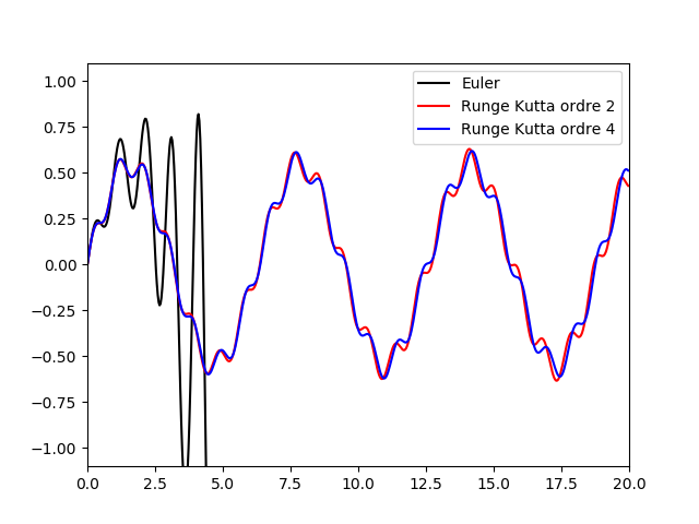
Exercise [Non Linear Equation of order $2$]
We want to solve this second order non linear differential equation:
\[
\left \{
\begin{array}{l}
ml^{2}\theta ^{\prime \prime }\left( t\right) =-mgl\sin \left( \theta \left(
t\right) \right) +c\left( t\right) \text{ pour }t\in \left[ 0,T\right] , \\
\theta \left( 0\right) =0 \\
\theta ^{\prime }\left( 0\right) =1.%
\end{array}%
\right.
\]
with torque $c\left( t\right) =A\sin \left( t\right) $, $m=0.1$kg,
$l=30$cm, $T=5$s and $A=0.1$N.m.
-
Solve this Cauchy problem with the Euler vector algorithm.
-
Solve this Cauchy problem with the Runge-Kutta of order $2$ algorithm.
-
Solve this Cauchy problem with the Runge-Kutta of order $4$ algorithm.
-
Solve this Cauchy problem with the second order Adams-Moulton algorithm.
import numpy as np

""" Euler Vector Algorithm"""

def F(t,V):
    L=[V[1], # TO DO]
    return np.array(L)

def NEuler(y0,a,b,nb):
    h=(b-a)/nb
    t=a
    X=[a]
    Y=[V0[0]]
    V1=V0
    for i in range(1,nb):
        #TO DO
        t=t+h
        Y.append(V2[0])
        X.append(t)
        V1=V2
    return X,Y
Exercise [Mass Spring]
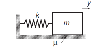
Consider the mass–spring system where dry friction is present between the block and the horizontal surface. The frictional force has a constant magnitude $\mu.m.g$ ($\mu$ is the coefficient of friction) and always opposes the motion. We denote by $y$ the measure from the position where the spring is unstretched.
We assume that $k = 3000$N/m, $\mu = 0.5$, $g = 9.80665$m/s², $y_0=0.1$m and $m= 6.0$ kg.- Write the differential equation of the motion of the block
- If the block is released from rest at $y = y_0$, verify by numerical integration that the next positive peak value of $y$ is $y_0 − 4\mu.m.\frac{g}{k}$. This relationship can be derived analytically.
Exercise [Iron block]
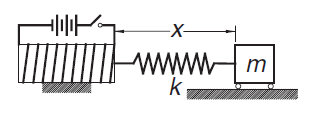
The magnetized iron block of mass $m$ is attached to a spring of stiffness $k$ and free length $L$. The block is at rest at $x = L$. When the electromagnet is turned on, it exerts a repulsive force $F = c/x^2$ on the block.
We assume that $c = 5$N·m², $k = 120$ N/m, $L = 0.2$m and $m= 1.0$ kg.- Write the differential equation of the motion of the mass
- Determine the amplitude and the period of the motion by numerical integration
Exercise [Magnus Effect applied to a ball]
On June 3, 1997, Roberto Carlos scored against France football team a free kick goal with an improbable effect.
We want to simulate in this exercice what happened that day. For this, we set:
- $\rho=1.2 \ Kg.m^{-3}$ : the air density
- $R=0.11\ m$ the radius of the ball
- $m = 0.430\ Kg$ : the mass of the ball
- $M(t)=(x(t),y(t),z(t))$: the location of the ball at $t\ge 0$
- $v_0=36 \ m.s^{-1}$ : the initial speed of the ball
- $v(t)$ : the speed of the ball at $t\ge 0$.
- $\overrightarrow{v}(t)$ : the speed vector of the ball at $t\ge 0$.
- $\overrightarrow{\omega}=(0,0,\omega_0)$ : the angular velocity of the ball which is assumed to be constant during the trajectory
- $\alpha$ : the angle between $\overrightarrow{\omega}$ and $\overrightarrow{v}$
- $\beta$, $\gamma$ : are the initial angles of the force applied to the ball
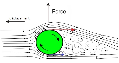 We assume that the forces applied to the ball are
- its weight
- a friction force: $\overrightarrow{f}$, $\Vert \overrightarrow{f} \Vert=\frac{1}{2}C_f\pi R^2\rho v^2,$ where $C_f\approx 0.45$
- a lift force $\overrightarrow{F}=\frac{1}{2}\pi\rho R^3\sin(\alpha)\ \overrightarrow{\omega}\wedge \overrightarrow{v}$.
-
Define the differential equation apply to the ball.
-
Define the initial conditions.
-
Solve this Cauchy problem with the Runge-Kutta of order $4$ algorithm.
-
Solve this Cauchy problem with the second order Adams-Moulton algorithm.
Runge-Kutta Algorithms
Runge-Kutta of order $2$We want to solve the following Cauchy problem: \[ \left\{ \begin{array} [c]{l}% y^{\prime}\left( t\right) =f\left( t,y\right) \\ y\left( t_{0}\right) =y_{0}% \end{array} \right. \text{ for }t\in\left[ t_{0},t_{n}\right] \] where $f$ is of class $C^{1}$. For this, we set \begin{align*} k_{1} & =h.f\left( t_{0},y_{0}\right) \\ k_{2} & =h.f\left( t_{0}+ah,y_{0}+\alpha k_{1}\right) \end{align*} and \[ y_{1}=y_{0}+R_{1}k_{1}+R_{2}k_{2}% \] Consequently, we have to calculate the unknows $a,\alpha,R_{1},R_{2}$ such that we minimize the following error: \[ e_{1}=y\left( t_{1}\right) -y_{1}% \] To do so, we identify the Taylor expansion of $y\left( t_{1}\right) $ and $y_{1}.$ We assume that $f$ is of class $C^{2}$. As \begin{align*} \frac{dy}{dt} & =f\left( t,y\right) \\ \frac{d^{2}y}{dt^{2}} & =\frac{\partial f\left( t,y\right) }{\partial t}+\frac{\partial f\left( t,y\right) }{\partial y}f\left( t,y\right) \end{align*} it yields, \begin{align*} y\left( t_{1}\right) & =y\left( t_{0}+h\right) \\ & \\ y\left( t_{1}\right) & =y_{0}+h.\frac{dy\left( t_{0}\right) }{dt}% +\frac{h^{2}}{2}\frac{d^{2}y\left( t_{0}\right) }{dt^{2}}+O\left( h^{3}\right) \\ & \\ y\left( t_{1}\right) & =y_{0}+h.f\left( t_{0},y_{0}\right) +\frac{h^{2}% }{2}\left[ \frac{\partial f\left( t_{0},y_{0}\right) }{\partial t}% +\frac{\partial f\left( t_{0},y_{0}\right) }{\partial y}f\left( t_{0}% ,y_{0}\right) \right] +O\left( h^{3}\right) \end{align*} As $\varphi\left(t,y,h\right) =R_{1}k_{1}+R_{2}k_{2}$ is of class $C^{2}$, we can apply the Taylor expansion at $h=0$. Then we have, \begin{align*} \varphi\left( t,y,h\right) & =\varphi\left( t,y,0\right) +h\frac {\partial\varphi\left( t,y,0\right) }{\partial h}+\frac{h^{2}}{2}% \frac{\partial^{2}\varphi\left( t,y,0\right) }{\partial h^{2}}+O\left( h^{3}\right) \\ \varphi\left( t,y,h\right) & =0+h\left[ R_{1}.f\left( t_{0}% ,y_{0}\right) \right] +h.\left[ R_{2}.f\left( t_{0},y_{0}\right) +R_{2}ha\frac{\partial f\left( t_{0},y_{0}\right) }{\partial t}\right] \\ & +h\left[ R_{2}h\alpha\frac{\partial f\left( t_{0},y_{0}\right) }{\partial y}f\left( t_{0},y_{0}\right) \right] +O\left( h^{3}\right) \end{align*} It comes \[ y_{1}=y_{0}+\left( R_{1}+R_{2}\right) hf\left( t_{0},y_{0}\right) \\ +h^{2}\left[ aR_{2}\frac{\partial f\left( t_{0},y_{0}\right) }{\partial t}+\alpha R_{2}\frac{\partial f\left( t_{0},y_{0}\right) }{\partial y}f\left( t_{0},y_{0}\right) \right] +O\left( h^{3}\right) . \] Then, the difference \begin{align*} y\left( t_{1}\right) -y_{1} & =\left( 1-R_{1}-R_{2}\right) hf\left( t_{0},y_{0}\right) +h^{2}\left[ \left( \frac{1}{2}-aR_{2}\right) \frac{\partial f\left( t_{0},y_{0}\right) }{\partial t}\right] \\ & +h^{2}\left[ \left( \frac{1}{2}-\alpha R_{2}\right) \frac{\partial f\left( t_{0},y_{0}\right) }{\partial y}f\left( t_{0},y_{0}\right) \right] +O\left( h^{3}\right) \end{align*} is of order $O\left( h^{3}\right) $ if $R_{1}+R_{2}=1$ and $aR_{2}=\alpha R_{2}=\dfrac{1}{2}.$ It follows that:
- if $R_{2}=0$ then we obtain the previous Euler method
- if $R_{1}=0,R_{2}=1$ and $a=\alpha=\dfrac{1}{2}$ we obtain the modified Euler method where $y_{1}=y_{0}+h.f\left( t_{0} +\frac{h}{2},y_{0}+\frac{h}{2}f\left( t_{0},y_{0}\right) \right) $
- if $R_{1}=R_{2}=\dfrac{1}{2}$ and $a=\alpha=1$ then we obtain the Euler-Cauchy method where $y_{1}=y_{0}+\dfrac{1}{2}hf\left( t_{0},y_{0}\right) +\dfrac{1}{2}h.f\left( t_{0}+h,y_{0}+hf\left( t_{0},y_{0}\right) \right) $.
The fourth-order Runge–Kutta method is obtained from the Taylor series along the samelines as the second-ordermethod. Since the derivation is rather long and not very instructive, we skip it. The final form of the integration formula again depends on the choice of the parameters; that is, there is no unique Runge–Kutta fourth-order formula. The most popular version, which is known simply as the Runge–Kutta method, entails the following sequence of operations: \begin{align*} k_{1} & =h.f\left( t_{0},y_{0}\right) \\ k_{2} & =h.f\left( t_{0}+\frac{h}{2},y_{0}+\frac{k_{1}}{2}\right) \\ k_{3} & =h.f\left( t_{0}+\frac{h}{2},y_{0}+\frac{k_{2}}{2}\right) \\ k_{4} & =h.f\left( t_{0}+h,y_{0}+k_{3}\right) \\ y_{1} & =y_{0}+\frac{1}{6}\left( k_{1}+2k_{2}+2k_{3}+k_{4}\right) \end{align*} The main drawback of this method is that it does not lend itself to an estimate of the truncation error. Therefore, we must guess the integration step size $h$, or determine it by trial and error. In contrast, the so-called adaptive methods can evaluate the truncation error in each integration step and adjust the value of $h$ accordingly (but at a higher cost of computation). The adaptive method is introduced in the next Section.
Multi-step Algorithms
For all $n$, we set $f\left( t_{n},y_{n}\right) =f_{n}.$ We call $k$-step method an algorithm of the kind: \[ \left\{ \begin{array} [c]{c}% y_{n}=\sum_{i=1}^{k}\alpha_{i}y_{n-i}+h \sum^{k}_{i=0}\beta_{i}f_{n-i}\text{ for }n\geq k\\ y_{0,}\ldots y_{k-1}\text{ are given} \end{array} \right. \] where the $\alpha_{i}$ and $\beta_{i}$ are real values which are not dependant of $h$.
- If $\beta_{0}=0$ then we have an explicit method.
- If $\beta_{0}\neq0$ then we have an implicit method.
If we integrate the differential equation we have: \[ y\left( t_{n}\right) =y\left( t_{n-1}\right) +\int_{t_{n-1}}^{t_{n}% }f\left( t,y\left( t\right) \right) dt \] In order to calculte this integral, we substitute $f\left( t,y\left( t\right) \right) $ by an interpolation polynomial $p\left( t\right) $ of degree $k$ which satisfies $p\left( t_{j}\right) =f\left( t_{j}% ,y_{j}\right) =f_{j}$ for $j=n-k,\ldots,n$. For this, we need to take into account the $k$ values $y_{n-k},\ldots,y_{n-1}$ that were calculated previously and $y_{n}$ which is known. If we write this polynomial in the Newton'polynomial basis we obtain: \[ y_{n}=y_{n-1}+\sum_{j=0}^{k}\left( \prod_{i=0}^{j-1}\left( t-t_{n-i}\right) f\left[ t_{n},\ldots,t_{n-j}\right] \right) . \] If the abscissa $t_{j}$ are uniform then it yields: \[ y_{n}=y_{n-1}+h\underset{i=0}{\overset{k}{\sum}}\beta_{i}f_{n-i}\text{.}% \] Coefficients $\beta_{i}$ have to be defined such that the formula are exacts for maximum degree polynomials. If $k=2$, \begin{align*} \text{for }y(t) & =1\text{ then }y^{\prime}(t)=0\text{ }\\ \text{and }y\left( t_{n}\right) & =1=y\left( t_{n-1}\right) +h.(f\left( t_{n},y_{n}\right) .\beta_{0}+f\left( t_{n-1},y_{n-1}\right) .\beta _{1}+f\left( t_{n-2},y_{n-2}\right) .\beta_{2})\\ \text{It yields }1 & =1+h.\left[ 0.\beta_{0}+0.\beta_{1}+0.\beta_{2}\right] \end{align*} \begin{align*} \text{for }y(t) & =t-t_{n}\text{ then }y^{\prime}(t)=1\\ \text{and }y\left( t_{n}\right) & =0=-h+h.(\beta_{0}+\beta_{1}+\beta_{2}) \end{align*} \begin{align*} \text{for }y(t) & =\left( t-t_{n}\right) ^{2}\text{ then }y^{\prime }(t)=2\left( t-t_{n}\right) \\ \text{and }y\left( t_{n}\right) & =0=h^{2}+h.(0.\beta_{0}-2h.\beta _{1}-4h.\beta_{2}) \end{align*} From \begin{align*} \beta_{0}+\beta_{1}+\beta_{2} & =1\\ 2.\beta_{1}-4.\beta_{2} & =1 \end{align*} we obtain that \begin{align*} \beta_{0} & =\beta_{1}=\frac{1}{2}\\ \beta_{2} & =0 \end{align*} Consequently, the Adams-Moulton of order $2$ can be written: \[ y_{n}=y_{n-1}+\frac{h}{2}\left( f_{n}+f_{n-1}\right) \] Order 3: \[ y_{n}=y_{n-1}+\frac{h}{12}\left( 5f_{n}+8f_{n-1}-f_{n-2}\right) \]
- To calculate $f_{n}$ we need to know the value $y_{n}$ then we have implicit methods. To solve then, we can approximate $y_{n}$ by $y_{n}^{\ast}$ by using an explicit method and insert this value in the implicit schema (correction step).
- Usually the implicit methods are more robust than the explicit ones.
Adams-Bashforth Algorithm
Order 2 :
\[
y_{n}=y_{n-1}+\frac{h}{2}\left( 3f_{n-1}-f_{n-2}\right)
\]
Order 3 :
\[
y_{n}=y_{n-1}+\frac{h}{12}\left( 23f_{n-1}-16f_{n-2}+5f_{n-3}\right)
\]
References
- Dennis, J.E., and Schnabel, R.B. 1983, Numerical Methods for Unconstrained Optimization and Nonlinear Equations; reprinted 1996 (Philadelphia: S.I.A.M.)