Two-Point Boundary Value Problems
Introduction
We consider boundary-value problems in which the conditions are specified at more than one point.
The crucial distinction between initial values problems and boundary value problems is that in the former case we are able to start
an acceptable solution at its beginning or initial values and just march it along by numerical integration to its end or final values.
A simple example of a second-order boundary-value problem is:
$$
(E) \left \{
\begin{array}
[ccc]{l}%
y''(x) & = & y(x) \\
y(0) & = & 0 \\ y(1) & = & 1 \\
\end{array}
\right.
$$
This is a classic exponential growth/decay problem where the exact solution to this two-point differential equation is:
$$
y(x)=\dfrac{e^x-e^{-x}}{e-\dfrac{1}{e}}
$$
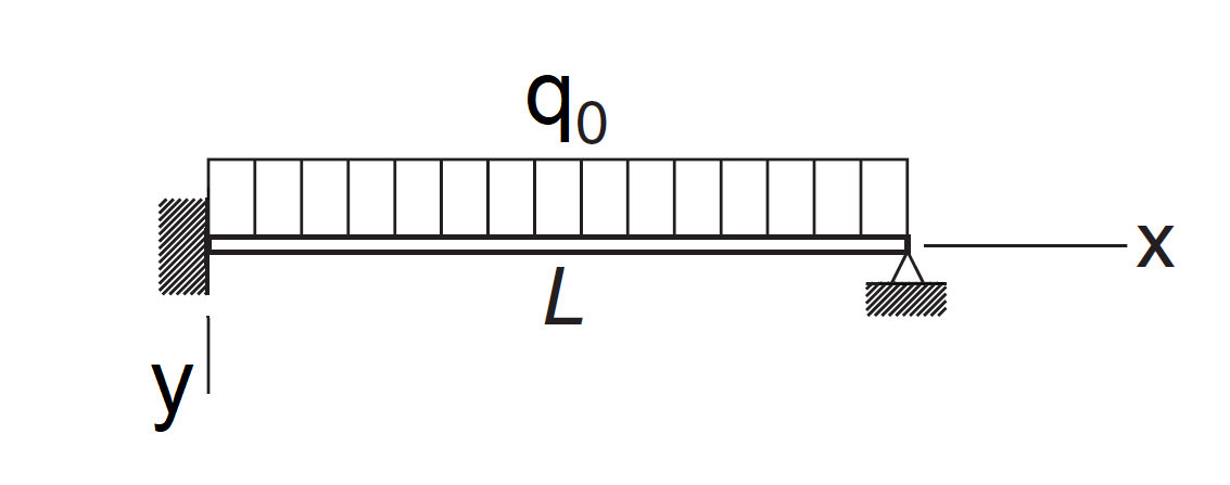
In the context of beam bending, we can have to solve a fourth-order system which has the form:
$$ y^{(4)}(x) +ky(x) = q_0 $$
with boundary conditions:
Here $y(x)$ represents the beam deflection at point $x$ along its length, $q_0$ represents a uniform load, and $L$ is the beam’s length. The first two boundary conditions say that the beam at $x = 0$ is rigidly attached. The second two boundary conditions say that the beam at $x = L$ is simply supported.
Finite Difference Method
In order to solve the previous two-point differential problems, we will use the finite difference method. For this, we firstly divide the range of integration $[a, b]$ into $m$ equal subintervals of length $h$ each, as shown in this Figure:
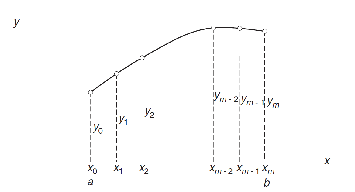
The values of the numerical
solution at the mesh points $x_i=a+ih$ are denoted by $y_i$ for $i = 0, 1, . . . ,m$ where $h=\dfrac{b-a}{m}$.
We now have to make two approximations:
- The derivatives of $y$ in the differential equations have to be replaced by their finite difference expressions (see below).
- The differential equations have to be enforced only at the mesh points.
The boundary conditions of the problem are fixed. Consequently, $y_0=y(0)=0$ and $y_m=y(1)=1$. They are exact. The interior mesh points $y_i$ for $i=1,...,m-1$ are then approximated. For this, we replace $y''(x_i)$ by its derivative approximation (See Exercice 1 ).
As a result, the differential equations are replaced by $m+1$ simultaneous algebraic equations where the unknowns are the $y_i$. If the differential equation is nonlinear, the algebraic equations will also be nonlinear and must be solved by the Newton–Raphson method.
Since the truncation error in a first central difference approximation is $\mathcal{O}(h^2)$, the finite difference method is not nearly as accurate as the shooting method—recall that the Runge–Kutta method has a truncation error of $\mathcal{O}(h^5)$. Therefore, the convergence criterion specified in the Newton–Raphson method should not be too severe.
Numerical Differentiation
In order to solve differential equations with boundaries conditions, we need to approximate the derivative terms. For this we use finite differences. Numerical differentiation deals with the following problem: we are given the function $y(x)$ and wish to obtain one of its derivatives at the point $x = x_i$. The term “given” means that we either have an algorithm for computing the function, or possess a set of discrete data points $(x_i , y_i )$, $i = 0, 1, . . . , m$. In either case, we have access to a finite number of $(x, y)$ data pairs from which to compute the derivative. If you suspect by now that numerical differentiation is related to interpolation, you are right—one means of finding the derivative is to approximate the function locally by a polynomial and then differentiate it. An equally effective tool is the Taylor series expansion of $y(x)$ about the point $x_i$, which has the advantage of providing us with information about the error involved in the approximation. Numerical differentiation is not a particularly accurate process. It suffers from a conflict between roundoff errors (due to limited machine precision) and errors inherent in interpolation. For this reason, a derivative of a function can never be computed with the same precision as the function itself. The derivation of the finite difference approximations for the derivatives of $y(x)$ is based on forward and backward Taylor series expansions of $y(x)$ about $x$, such as
$$ \left \{ \begin{array} [c]{l}% y(x_i + h) = y(x_i) + hy^{(1)}(x_i) + \dfrac{h^2}{2!}y^{(2)}(x_i) + \dfrac{h^3}{3!}y^{(3)}(x_i)+ \dfrac{h^4}{4!}y^{(4)}(x_i) + \mathcal{O}(h^4)\\ y(x_i - h) = y(x_i) - hy^{(1)}(x_i) + \dfrac{h^2}{2!}y^{(2)}(x_i) - \dfrac{h^3}{3!}y^{(3)}(x_i)+ \dfrac{h^4}{4!}y^{(4)}(x_i) + \mathcal{O}(h^4)\\ \end{array} \right. $$ A Taylor series is meaningful only if all the derivatives of $y(x)$ exist at $x=x_i$ and the series converges. In general, convergence occurs only if $x$ is sufficiently close to $x_i$ i.e. if $|h| < \varepsilon$, where $\varepsilon$ is called the radius of convergence. We also record the sums and differences of the series: $$ \left \{ \begin{array} [c]{l}% y(x_i + h) - y(x_i - h) = 2hy^{(1)}(x_i) + \dfrac{h^3}{3}y^{(3)}(x_i) + \mathcal{O}(h^3)\\ y(x_i + h) + y(x_i - h) = 2y(x_i) + h^2y^{(2)}(x_i) + \dfrac{h^4}{12}y^{(4)}(x_i) +\mathcal{O}(h^4)\\ \end{array} \right. $$ Note that the sums contain only even derivatives, whereas the differences retain just the odd derivatives. These equations can be viewed as simultaneous equations that can be solved for various derivatives of $y(x)$. The number of equations involved and the number of terms kept in each equation depend on the order of the derivative and the desired degree of accuracy.
First Central Difference Approximations
The solutions of $y^{(1)}(x_i)$ and $y^{(2)}(x_i)$ are:
$$
\left \{
\begin{array}
[c]{l}%
y^{(1)}(x_i) = \dfrac{y(x_i+h)-y(x_i-h)}{2h}+\mathcal{O}(h^2) \\
y^{(2)}(x_i) = \dfrac{y(x_i+h)-2y(x_i)+y(x_i-h)}{h^2}+\mathcal{O}(h^2) \\
\end{array}
\right.
$$
which is called the first and second central differences approximations for $y(x)$ at $x_i$. The term $\mathcal{O}(h^2)$
reminds us that the truncation error behaves as $h^2$.
Consequently, by denoting $y_i$ the approximation of $y(x_i)$, $y_{i+1}$ the approximation of $y(x_i+h)$ ...
and by forgetting the term $\mathcal{O}(h^2)$, we obtain the following approximations:
$$
\left \{
\begin{array}
[c]{l}%
y^{(1)}_i = \dfrac{y_{i+1}-y_i}{2h} \\
y^{(2)}_i = \dfrac{y_{i+1}-2y_i+y_{i-1}}{h^2} \\
\end{array}
\right.
$$
Central difference approximations for other derivatives can be obtained in the same manner.
First Noncentral Finite Difference Approximations
Central finite difference approximations are not always usable. For example, consider
the situation where the function is given at the $n$ discrete points $x_0, x_1, . . . , x_n$.
Since central differences use values of the function on each side of $x$, we would
be unable to compute the derivatives at $x_0$ and $x_n$. Clearly, there is a need for finite
difference expressions that require evaluations of the function only on one
side of $x$. These expressions are called forward and backward finite difference
approximations.
Noncentral finite differences can also be obtained from
$$
y^{(1)}(x_i) = \dfrac{y(x_i+h)-y(x_i)}{h} - \dfrac{h}{2}y^{(2)}(x_i) - \dfrac{h^2}{6}y^{(3)}(x_i) + \mathcal{O}(h^2)
$$
Keeping only the first termon the right-hand side leads to the first forward difference approximation
$$
y^{(1)}(x_i) = \dfrac{y(x_i+h)-y(x_i)}{h} + \mathcal{O}(h)
$$
Similarly, we obtain the first backward difference approximation:
$$
y^{(1)}(x_i) = \dfrac{y(x_i)-y(x_i-h)}{h} + \mathcal{O}(h)
$$
Note that the truncation error is now $\mathcal{O}(h)$, which is not as good as $\mathcal{O}(h^2)$ in central difference approximations.
We can derive the approximations for higher derivatives in the same manner:
$$
y^{(2)}(x_i) = \dfrac{y(x_i+2h)-2y(x_i+h)+y(x_i)}{h^2} + \mathcal{O}(h)
$$
We then obtain the following approximations:
$$
\left \{
\begin{array}
[c]{l}%
y^{(1)}_i = \dfrac{y_i-y_{i-1}}{h} \\
y^{(2)}_i = \dfrac{y_{i+2}-2y_{i+1}+y_i}{h^2}
\end{array}
\right.
$$
Errors in Finite Difference Approximations
Observe that in all finite difference expressions the sum of the coefficients is zero.
The effect on the roundoff error can be profound. If his very small, the values of $y(x)$,
$y(x ± h)$, $y(x ± 2h)$... will be approximately equal. When they are multiplied by the
coefficients and added, several significant figures can be lost. On the other hand, we
cannot make $h$ too large, because then the truncation error would become excessive.
This unfortunate situation has no remedy, but we can obtain some relief by taking
the following precautions:
- Use double-precision arithmetic.
- Employ finite difference formulas that are accurate to at least $\mathcal{O}(h^2)$.
To illustrate the errors, let us compute the second derivative of $y(x) = e^{−x}$ at $x = 1$
from the central difference formula. We carry out the calculations with double-digit precision, using different values of $h$.
The results, shown in the following Table,
are compared with $y^{(2)}(1) = e^{−1} =$ 0.367 879 441 171 442
| $h=0.64 \times 2^{-3i}$ | approximation value | error |
| 0.64 | 0.380 609 096 726 167 | 1.272965e-02 |
| 0.08 | 0.368 075 685 401 340 | 1.962442e-04 |
| 0.01 | 0.367 882 506 843 719 | 3.065672e-06 |
| 0.00125 | 0.367 879 489 040 490 | 4.786904e-08 |
| 0.000 156 25 | 0.367 879 438 272 211 | 2.899230e-09 |
| 1.953125e-05 | 0.367 879 401 892 423 | 3.927901e-08 |
| 2.44140625e-06 | 0.367 872 416 973 114 | 7.024198e-06 |
| 3.0517578125e-07 | 0.367 164 611 816 406 | 7.148293e-04 |
As we can see, the error is non linear with $h$. There exits an optimal value $h^*$ such that the error is minimal.
The Shooting Method
An another methodoly to solve the two-point boundary problems is to used a shooting methodology. The basic idea of the shooting method is this: Instead of tying a general solution to a boundary value problem down at both points, one only ties it down at one end. In the case of a second order problem, this leaves a free parameter. For a given value of this free parameter, one then integrates out a solution to the differential equation. Specifically, you start at the tied-down boundary point and integrate out just like an initial value problem. When you get to the other boundary point, the error between your solution and the true boundary condition tells you how to adjust the free parameter. Repeat this process until a solution matching the second boundary condition is obtained. The shooting method tend to converge very quickly and it also works for non-linear differential equations. The disadvantage is that convergence is not guaranteed. To begin, given a boundary value problem:
$$ \left \{ \begin{array} [ccc]{l}% y''(x) & = & f(x,y,y') \\ y(a) & = & \alpha \\ y(b) & = & \beta \\ \end{array} \right. $$The idea is to find the absent initial value $y′(a)$ that would enable $y$ to attain the $\beta$ value at $x = b$. We then transform the previous problem into the following initial value problem: $$ \left \{ \begin{array} [ccc]{l}% y''(x) & = & f(x,y,y') \\ y(a) & = & \alpha \\ y'(a) & = & s \\ \end{array} \right. $$ For each initial value $s$ for $y′(a)$, the initial value problem in general has a unique solution denoted by $y_s(x)$. So the original boundary value problem reduces to finding a zero $s^*$ of the function: $$ F(s) = y_s(b) − β $$
Exercice 1.
$$ \left \{ \begin{array} [ccc]{l}% y''(x) & = & y(x) \\ y(0) & = & 0 \\ y(1) & = & 1 \\ \end{array} \right. $$
We want to solve this problem with the finite difference method for a given value $m$. We then have $h=\dfrac{1}{m}$.
- By using the second order central finite difference approximation show that this problem yields the following algebraic equations: $$ \left \{ \begin{array} [ccccc]{r}% \dfrac{1}{h^2}y_{i+1} - (1 + \dfrac{2}{h^2})y_i + \dfrac{1}{h^2}y_{i-1} & = & 0 & for & i=1,...,m-1\\ y_0 & = & 0 \\ y_m & = & 1 \\ \end{array} \right. $$
- By taking the boundary conditions, show that we have to solve a $m \times m$ linear system.
$$ \left[\begin{array}{ccccc} 1 + \dfrac{2}{h^2} & -\dfrac{1}{h^2} & 0 & \ldots & 0\\ -\dfrac{1}{h^2} & 1 + \dfrac{2}{h^2} & -\dfrac{1}{h^2} & \ddots & \vdots\\ 0 & \ddots & \ddots & \ddots & 0 \\ \vdots & \ddots & -\dfrac{1}{h^2} & 1 + \dfrac{2}{h^2} & -\dfrac{1}{h^2} \\ 0 & \ldots & 0 & -\dfrac{1}{h^2} & 1 + \dfrac{2}{h^2} \\ \end{array}\right] \left[\begin{array}{c} y_1\\ y_2\\ \vdots\\ \vdots\\ \vdots\\ y_{m-2}\\ y_{m-1} \end{array}\right] =\qquad \left[\begin{array}{c} 0\\ 0\\ \vdots\\ \vdots\\ \vdots\\ 0\\ \dfrac{1}{h^2}\\ \end{array}\right] $$ where the $y_i$ for all $i=1,...,m-1$ are the unknows of the problem. - Solve this linear system with Python and compare the so obtained solution with the exact solution (see Introduction )
- Calculate the maximum error according to the value of $m$.
import numpy as np
from numpy import linalg as LA

def FiniteDifference(m)
    A = np.zeros((m-1,m-1),dtype = np.float64)
    b = np.zeros((m-1), dtype = np.float64)
    h=1/m
    a=(1+2/(h*h))
    c=-1/(h*h)
    """ Definition of the matrix """
    for i in range(m-1):
        for j in range(m-1):
            if i==j:
                A[i,j]=a
            if i==j+1 or i==j+1:
                A[i,j]=c
    b[m-2]=c
    X = LA.solve(A,b)
    X = np.append(X,1)
    X = np.insert(X,0,0)
    return X

def f(x)
    # To do
    return


m = 10
y = FiniteDifference(m)
x = np.linspace(0,1,m+1)
Y = f(x)
err = np.abs(Y-y)
err = np.delete(err,0)
err = np.delete(err,m-1)
print("min error= ",np.min(err)," max error= ",np.max(err))
| $x_i$ | $y_i$ | $y(x_i)$ |
| 0.0 | 0.0 | 0.0 |
| 0.1 | 0.085 244 69 | 0.085 233 70 |
| 0.2 | 0.171 341 82 | 0.171 320 45 |
| 0.3 | 0.259 152 38 | 0.259 121 84 |
| 0.4 | 0.349 554 46 | 0.349 516 60 |
| 0.5 | 0.443 452 08 | 0.443 409 44 |
| 0.6 | 0.541 784 22 | 0.541 740 07 |
| 0.7 | 0.645 534 21 | 0.645 492 62 |
| 0.8 | 0.755 739 53 | 0.755 705 48 |
| 0.9 | 0.873 502 26 | 0.873 481 69 |
| 1.0 | 1.0 | 1.0 |
As we can see in this Table, for $m=10$, the minimum/maximum errors are about $1.09\ 10^{-5}$ and $4.414\ 10^{-5}$. We obtain for $m=100$ that the maximum error is about $4.4219\ 10^{-7}$
Exercice 2.
Let us given the following linear boundary value problem defined on $[0,\dfrac{\pi}{2}]$: $$ \left \{ \begin{array} [ccc]{lcl}% y''(x) & = & 4x - 4y(x) \\ y(0) & = & 0 \\ y'(\dfrac{\pi}{2}) & = & 1 \end{array} \right. $$ We want to solve this problem with the finite difference method with a given value of $m$ and consequently $h$.
Write the linear system that we have to solve knowing the value of $h$. For this, you have to use the first backward difference approximation to deal with the second boundary condition. You have to use the central difference approximation in the interior mesh points.
- Solve numerically this problem with different values of $m$.
-
According to given values of $m$, calculate the maximum error between the approximated solution and the exact solution of this problem $y(x) = x -sin(2x)$.
Exercice 3. "Beam deflection"
We consider in this exercice the following problem:
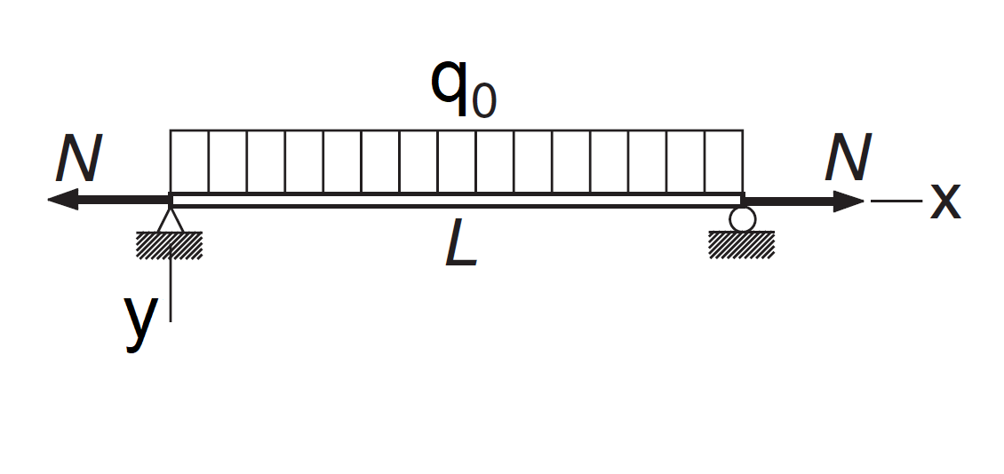 This beam carries a uniform load of intensity $q_0$ and the tensile
force $N$. The differential equation for the vertical displacement $y$ can be shown
to be:
\[
\dfrac{d^4y}{dx^4}(x) - \dfrac{N}{EI}\dfrac{d^2y}{dx^2}(x)= \dfrac{q_0}{EI}
\]
where $EI$ is the bending rigidity. The boundary conditions are
\[
\begin{array}{ccc}
\left \{
\begin{array}{cccc}
y(0) & = & 0 \\
\dfrac{d^2y}{dx^2}(0) & = & 0 \\
\end{array}
\right. & & &
\left \{
\begin{array}{ccc}
y(L) & = & 0 \\
\dfrac{d^2y}{dx^2}(L) & = & 0 \\
\end{array}
\right.
\end{array}
\]
Changing the variables to $u = \dfrac{x}{L}$ and $v = y.\dfrac{EI}{q_0L^4}$ transforms
the problem to the dimensionless form
\[
\dfrac{d^4v}{du^4}(u) - \beta \dfrac{d^2v}{du^2}(u) = 1
\]
where $\beta = \dfrac{NL^2}{EI}$ and $v(0)=\dfrac{d^2v}{du^2}(0) = v(1)=\dfrac{d^2v}{du^2}(1) = 0$.
This beam carries a uniform load of intensity $q_0$ and the tensile
force $N$. The differential equation for the vertical displacement $y$ can be shown
to be:
\[
\dfrac{d^4y}{dx^4}(x) - \dfrac{N}{EI}\dfrac{d^2y}{dx^2}(x)= \dfrac{q_0}{EI}
\]
where $EI$ is the bending rigidity. The boundary conditions are
\[
\begin{array}{ccc}
\left \{
\begin{array}{cccc}
y(0) & = & 0 \\
\dfrac{d^2y}{dx^2}(0) & = & 0 \\
\end{array}
\right. & & &
\left \{
\begin{array}{ccc}
y(L) & = & 0 \\
\dfrac{d^2y}{dx^2}(L) & = & 0 \\
\end{array}
\right.
\end{array}
\]
Changing the variables to $u = \dfrac{x}{L}$ and $v = y.\dfrac{EI}{q_0L^4}$ transforms
the problem to the dimensionless form
\[
\dfrac{d^4v}{du^4}(u) - \beta \dfrac{d^2v}{du^2}(u) = 1
\]
where $\beta = \dfrac{NL^2}{EI}$ and $v(0)=\dfrac{d^2v}{du^2}(0) = v(1)=\dfrac{d^2v}{du^2}(1) = 0$.
We want to solve this problem with the finite difference method.
-
Define the central finite difference scheme for the fourth order derivative. Use the forward and backward difference approximations at the boundaries. You have to use the central difference approximation in the interior mesh points.
- Calculate the linear system obtained for a given $m$.
- Determine the maximum displacement for $\beta = 1.65929$. Plot the solution.
- Determine the maximum displacement for $\beta = −1.65929$. This case means that $N$ is compressive.
Exercice 4. "Heat equation"
 Casting is a process in which a liquid metal is somehow delivered into a mold. The heat equation is a partial differential equation
that describes how the distribution of heat evolves over time in a solid medium,
as it spontaneously flows from places where it is higher towards places where it is lower.
This equation was first developed and solved by Joseph Fourier in 1822 to describe heat flow.
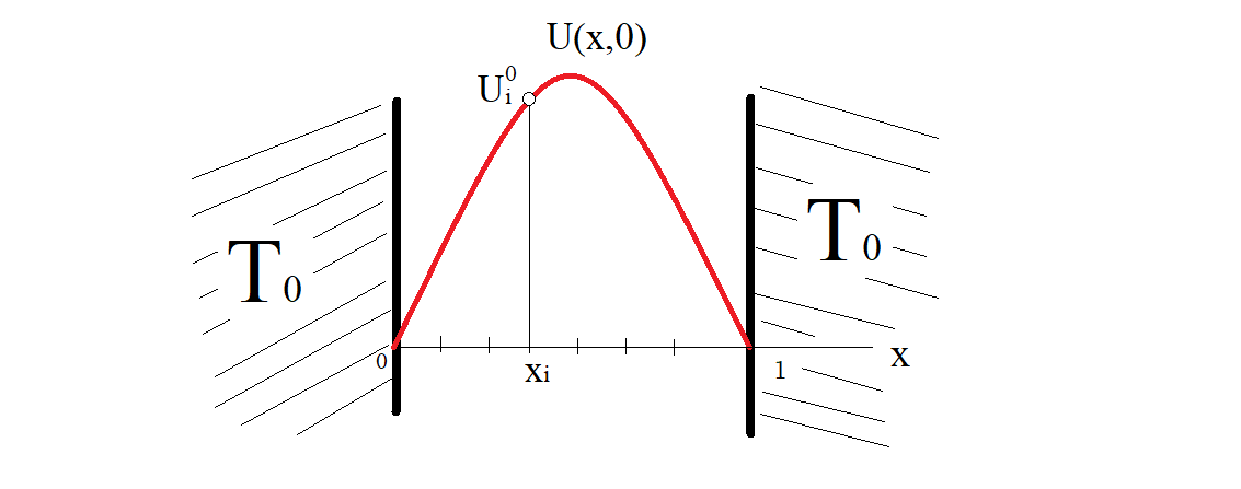
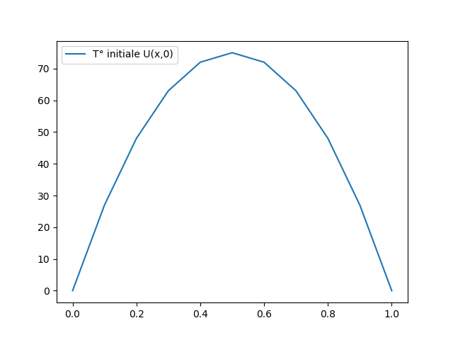
In this Figure, we assume that the temperature of the air or in the sand part is $T_0=0$.
The red curve is the temperature $U(x,0)$ of the liquid metal inside the mold at the initial state.
Let us given $x_i$, we want to calculate an approximation $U_i^j$ of the evolution of the temperature inside the mold in order
to know when the metal will be in his "solid" state.
The upper index $j$ in $U_i^j$ represents the step time $t_j$, $j=0$ or $t_0$ being the initial time.
Casting is a process in which a liquid metal is somehow delivered into a mold. The heat equation is a partial differential equation
that describes how the distribution of heat evolves over time in a solid medium,
as it spontaneously flows from places where it is higher towards places where it is lower.
This equation was first developed and solved by Joseph Fourier in 1822 to describe heat flow.
In this Figure, we assume that the temperature of the air or in the sand part is $T_0=0$.
The red curve is the temperature $U(x,0)$ of the liquid metal inside the mold at the initial state.
Let us given $x_i$, we want to calculate an approximation $U_i^j$ of the evolution of the temperature inside the mold in order
to know when the metal will be in his "solid" state.
The upper index $j$ in $U_i^j$ represents the step time $t_j$, $j=0$ or $t_0$ being the initial time.
For this, we need to solve the following heat equation with boundary conditions:
\[
\left \{
\begin{array}
[c]{l}%
\dfrac{\partial U}{\partial t}\left( x,t\right) =\alpha \dfrac{\partial^{2}%
U}{\partial x^{2}}\left( x,t\right) \text{ for }x\in \left] 0,1\right[ \\
U\left( 0,t\right) =U\left( 1,t\right) =0\text{ for all }t>0\\
U\left( x,0\right) =300x\left( 1-x\right)
\end{array}
\right.
\]
where $\alpha$ is the thermal diffusivity. It has the SI derived unit of $m^{2}/s$.
The initial temperature in the medium is given by $U\left( x,0\right)$. The temperature at $x=0=1$ is assumed to be equal to $0$ for all $t\geq 0$.
-
By denoting $U_i^j$ the approximation of the temperature $U\left( x_{i},t_{j}\right)$ in the liquid metal at $x_i$ for time $t_j$, write the finite difference scheme of the heat equation. For this, you have to use the central finite difference for the space $x$ variable and the forward finite difference for time $t$ variable. We assume that $x_{i}=ih$ for $i=0,...,m$ with $h=\dfrac{1}{m}$ and $t_{j}=j\Delta t$.
As $U^{j}_0=U^{j}_m=0$ for any $j\geq 0$, we then have for any $i=1,..,m-1$: $$ \dfrac{U^{j+1}_i-U^j_i}{\Delta t}=\alpha \dfrac{U^{j}_{i+1}-2U^{j}_i+U^{j}_{i-1}}{h^2} $$ It yields: $$ U^{j+1}_i = U^{j}_i + r U^{j}_{i+1} - 2r U^{j}_i + rU^{j}_{i-1} $$ where $r=\alpha \dfrac{\Delta t}{h^{2}}$. - Write this scheme in the follwoing form: \[ U^{\left( j+1\right) }=(\mathbf{I}+r\mathbf{A})U^{\left( j\right) }% \] where matrix $\mathbf{A}$ has to be defined and the vectors $U^{\left( j\right) }=\left( U_{1}^{j},...,U_{p-1}^{j}\right) ^{T}$ denote the temperature at each step time $t_{j}$ in the medium. Solve this linear system at each step time and draw all this temperature profiles.
-
According to the values of $h$ and $\Delta t$ the solution may diverge. For example, with $\alpha=0.01$, $m=10$ and $\Delta=1$ the solution is unstable as we can see in the following Figure:
$$ \dfrac{1}{2} \left( \dfrac{U^{j}_{i+1}-2U^{j}_i+U^{j}_{i-1}}{h^2} + \dfrac{U^{j+1}_{i+1}-2U^{j+1}_i+U^{j+1}_{i-1}}{h^2} \right) $$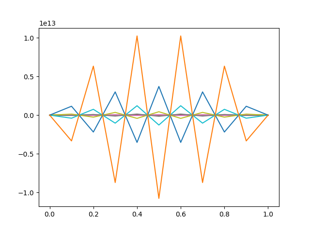 Loosely speaking, a method of numerical integration is said to be stable if the effects
of local errors do not accumulate catastrophically; that is, if the global error remains
bounded. If the method is unstable, the global error will increase exponentially, eventually
causing numerical overflow. Stability has nothing to do with accuracy; in fact,
an inaccurate method can be very stable.
To avoid this problem we want to solve the system by using the
Crank-Nicolson's scheme where we substitute the second partial derivative in $x$ by:
Loosely speaking, a method of numerical integration is said to be stable if the effects
of local errors do not accumulate catastrophically; that is, if the global error remains
bounded. If the method is unstable, the global error will increase exponentially, eventually
causing numerical overflow. Stability has nothing to do with accuracy; in fact,
an inaccurate method can be very stable.
To avoid this problem we want to solve the system by using the
Crank-Nicolson's scheme where we substitute the second partial derivative in $x$ by:
Apply this scheme and draw the temperature evolution in the medium at each time step. With the same values: $\alpha=0.01$, $m=10$ and $\Delta=1$ we obtain the stable solution where each curve represents the temperature in the mold at each step time $t_j$:
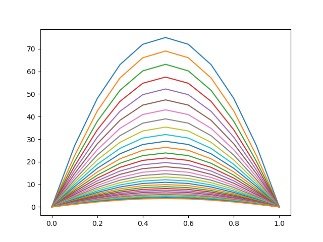
We have to solve at each time step $t_j$ the following linear system: \[ (\mathbf{I}-\frac{r}{2}\mathbf{A})U^{\left( j+1\right) }=(\mathbf{I}+\frac{r}{2}\mathbf{A})U^{\left( j\right) }% \]
- We want to see if this scheme is stable whatever the choice of $h$ and $\Delta t$. For this, show that: $$ U^{\left( j+1\right) } = \mathbf{P}^{j+1}U^{\left( 0\right) } $$ where $\mathbf{P}$ is a symmetric matrix. Then, calculate the eigenvalues of $\mathbf{P}$ by using the python numpy.linalg.eig function and conclude.
-
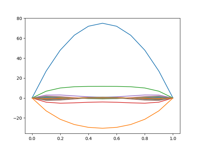
The approximate solutions can still contain (decaying) spurious oscillations if the ratio of time step $\Delta$ times the thermal diffusivity to the square of space step, $h^2$, is large. For this reason, whenever large time steps or high spatial resolution is necessary, the less accurate backward Euler method is often used, which is both stable and immune to oscillations. Try to see, if you have such spurious oscillations. In the following example, the method converges but the temperature becomes negative in some points which is not physically possible:
Exercice 5. "String Vibration"
We wish to solve the differential equation of a vibrating string of constant linear mass $\mu$ subjected to a tension $T$. One supposes that the weight of the string is negligible as well as all the causes of dampings in front of the tension forces. The string is supposed to be pinched at its ends. \[ \left \{ \begin{array} [c]{l}% \dfrac{\partial^{2}U}{\partial x^{2}}\left( x,t\right) -\dfrac{1}{c^{2}% }\dfrac{\partial^{2}U}{\partial t^{2}}\left( x,t\right) =0\\ U\left( 0,t\right) =U\left( 1,t\right) =0\text{ for all }t>0\\ U\left( x,0\right) =f\left( x\right) \\ \dfrac{\partial U}{\partial t}\left( x,0\right) =g\left( x\right) \end{array} \right. \text{ for all }x\in \left[ 0,1\right] \] where $c=\sqrt{\frac{T}{\mu}}$ is the wave velocity in the string. The value $U\left( x,t\right)$ is the vibration amplitude of the string at $x$ and $t$. We denote by $U^j_i$ its approximation. Consequently we have to solve this system for $x\in \left[ 0,1\right] $ and $t>0$. We assume that function $f$ is of class $C^{2}$ and function $g$ is of class $C^{1}$ on $\left[ 0,1\right]$.
-
Discretized this equation at each $x_{i}=ih$ for all $i=0,\ldots,m$. We assume that $h=\dfrac{1}{m}$ and $t_{j}=j\Delta t$. Write the linear system obtained by using a central point finite difference method for the space $x$ variable and a forward finite difference method for the time variable. Write this system on the following form: $$\mathbf{A}U^{\left( j+2\right) }=\mathbf{B}U^{\left( j+1\right) }+\mathbf{C}U^{\left( j\right) }$$ where vector $U^{\left( j\right) }$ is the vibration amplitude of the string at each time step $t_{j}$. We use a forward finite difference method to deal with the initial derivative condition.
As $U^{j}_0=U^{j}_m=0$ for any $j\geq 0$, we then have for any $i=1,..,m-1$: $$ \dfrac{U^{j+2}_i-2U^{j+1}_i+U^{j}_i}{\Delta t^2}=c^2 \dfrac{U^{j}_{i+1}-2U^{j}_i+U^{j}_{i-1}}{h^2} $$ It yields: $$ U^{j+2}_i = 2U^{j+1}_i + r U^{j}_{i+1} -(1 + 2r) U^{j}_i + rU^{j}_{i-1} $$ where $r=\left(\dfrac{c \times \Delta t}{h}\right)^2$. To start the iterations, we then need to know the two vectors $U^{\left( 0\right)}$ and $U^{\left( 1\right)}$. For this, we use the following condition: $\dfrac{\partial U}{\partial t}\left( x,0\right) =g\left( x\right)$. It yields the following approximation: $$ \dfrac{U^{1}_i-U^{0}_i}{\Delta t} = g(x_i) $$ Hence, $U^{1}_i = U^{0}_i + \Delta t \times g(x_i)$, which allows us to initialize the $U^{\left( 1\right)}$ vector. The $U^{\left( 0\right)}$ vector is initialized with $f(x_i)$. Consequently, $\mathbf{A} = \mathbf{I}$, $\mathbf{B} = 2\mathbf{I}$ and $\mathbf{C}$ is a tridiagonal matrix. -
We set $f(x)=x^{2}(1-x)$ and $g(x)=x(1-x)$. Solve each linear systems at each step time. We assume that $c=1$ and $m=100$.
- Draw the string evolution at each time step.
- Apply a Crank-Nicholson scheme type to this system. Conclude.
References
- J. Stoer and R. Bulirsch (1993), Introduction to Numerical Analysis. Springer-Verlag New York, Inc., 2nd edition
- S. D. Conte and Carl de Boor (1972), Elementary Numerical Analysis. McGraw-Hill, Inc., 2nd edition.
- F. B. Hildebrand (1968), Finite-difference Equations and Simulations. Prentice-Hall.