Polynomial Interpolation
- Introduction
- Canonical Interpolation
- Lagrange Interpolation
- Divided differences of a function
- Newton Interpolation
- Interpolation Polynomial Errors
- Sensibility of the solution to roundoff errors
- Cubic Spline Interpolation
Introduction
Discrete data sets, or tables of the form $$ \begin{array}{|c|c|c|c|c|c|} \hline & j=1 & j=2 & j=3 & \ldots & j=p \\ \hline x_j & x_1 & x_2 & x_3 & \ldots & x_p \\ \hline y_j & y_1 & y_2 & y_3 & \ldots & y_p \\ \hline \end{array} $$ are commonly involved in technical calculations. We assume that $x_1 < x_2 < \ldots < x_p$. The source of the data may be experimental observations or numerical computations. There is a distinction between interpolation and curve fitting. In interpolation, we construct a polynomial curve through the data points. In doing so, we make the implicit assumption that the data points are accurate and distinct.
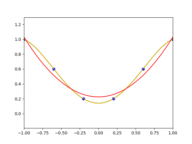
Curve fitting is applied to data that contain scatter (noise), usually due to
measurement errors. Here we want to find a smooth polynomial curve that approximates the data
in some sense. Thus the curve does not necessarily hit the data points. The difference
between interpolation and polynomial curve fitting is illustrated in the following figure:
We denote by $\cal{P}_n$ the linear space of polynomials of degree $\leq n$.
Canonical Interpolation Problem
We want to define a continuous curve which goes through all points without a break or a kink. The problem is that there are an infinite number of curves that go smoothly though the points, and unless we can define what the French curve (or the artistic hand) does in a precise mathematical way, the computer is stuck.
For this, we use polynomial interpolation. It is often needed to estimate the value of a function $y=f(x)$ at
certan point $x$ based on the known values of the function
$f(x_0),\cdots,f(x_n)$ at a set of node points $a=x_0\le x_1\le\cdots\le x_n=b$ in the interval $[a,\; b]$.
This process is called interpolation if $a \le x\le b$ or extrapolation if either
$x< a$ or $b< x$. One way to carry out these operations is to approximate the function $f(x)$ by an $n$-th degree polynomial:
\begin{equation}
f(x)\approx P_n(x)=a_0 + a_1x+ a_2x^2+ \cdots+a_{n-1}x^{n-1}+a_nx^n
=\sum_{j=0}^n a_jx^j
\end{equation}
where the $n+1$ coefficients $a_0,\cdots,a_n$ can be obtained based
on the given points. Once $P_n(x)$ is available, any operation
applied to $f(x)$, such as differentiation, intergration, and root
finding, can be carried out approximately based on
$P_n(x)\approx f(x)$.
This is particulary useful if $f(x)$ is non-elementary and therefore
difficult to manipulate, or it is only available as a set of discrete
samples without a closed-form expression.
Specifically, to find the coefficients of $P_n(x)$, we require it to pass through all node points $\{x_i,y_i=f(x_i),\;i=0,\cdots,n\}$, i.e. the following $n+1$ linear equations hold: \begin{equation} P_n(x_i)=\sum_{j=0}^n a_jx^j_i=f(x_i)=y_i,\;\;\;\;(i=0,\cdots,n) \end{equation} Now the coefficients $a_0,\cdots,a_n$ can be found by solving these $n+1$ linear equations, which can be expressed in matrix form as: \begin{equation} \left[ \begin{array}{ccccc} 1 & x_0 & x_0^2 & \cdots & x_0^n \\ 1 & x_1 & x_1^2 & \cdots & x_1^n \\ 1 & x_2 & x_2^2 & \cdots & x_2^n \\ \vdots & \vdots & \vdots & \ddots & \vdots \\ 1 & x_n & x_n^2 & \cdots & x_n^n \end{array}\right] \left[\begin{array}{c}a_0\\a_1\\a_2\\\vdots\\a_n\end{array}\right] =\left[\begin{array}{c}y_0\\y_1\\y_2\\\vdots\\y_n\end{array}\right] ={\bf b} \end{equation} where ${\bf x}=[a_0,\cdots,a_n]^T$, ${\bf b}=[y_0,\cdots,y_n]^T$ and \begin{equation} {\bf A}=\left[ \begin{array}{ccccc} 1 & x_0 & x_0^2 & \cdots & x_0^n \\ 1 & x_1 & x_1^2 & \cdots & x_1^n \\ 1 & x_2 & x_2^2 & \cdots & x_2^n \\ \vdots & \vdots & \vdots & \ddots & \vdots \\ 1 & x_n & x_n^2 & \cdots & x_n^n \end{array}\right] \end{equation} is known as the Vandermonde matrix. Solving this linear equation system, we get the coefficients $[a_0,\cdots,a_n]^T={\bf x}={\bf A}^{-1}{\bf b}$. Here $n+1$ polynomials $x^0, x^1, x^2,\cdots,x^n$ can be considered as a set of polynomial basis functions that span the space of all nth degree polynomials (which can also be spanned by any other possible bases). If the node points $x_0,\cdots,x_n$ are distinct, i.e., ${\bf A}$ has a full rank and its inverse ${\bf A}^{-1}$ exists, then the solution of the system ${\bf x}={\bf A}^{-1}{\bf b}$ is unique and so is $P_n(x)$.
In practice, however, this method is not widely used for two reasons: (1) the high computational complexity $O(n^3)$ for calculating ${\bf A}^{-1}$, and (2) matrix ${\bf A}$ becomes more ill-conditioned as $n$ increases. Instead, other methods to be discussed in the following section are practically used.
Exercice [PY-1]
We want to interpolate the following data by using a polynomial function with the appropriate degree $$ \begin{array}{|c|c|c|c|c|} \hline -1.0 & -\frac{1}{2} & 0.0 & \frac{1}{2} & 1.0 \\ \hline 1.0 & \frac{1}{2} & 0.0 & \frac{1}{2} & 1.0 \\ \hline \end{array} $$
-
Let $$P_{n}\left(x\right)=\sum_{i=0}^{n}a_{i}x^{i}$$ be a polynomial function. Write the linear system which allows to the function to interpolate the previous data. Choose the appropriate value for $n$.
-
Solve this system by using the linalg library of numpy.
-
Define the Pol(x,coeff) function which return for a given $x$ the value of the polynomial function for which the coefficients are given in the coeff list. You can use the Horner algorithm.
-
By using X=np.linspace(a,b,p) which generates uniform p-values between $a=-1$ and $b=1$, draw the previous polynomial function. You can use the list t=np.linspace(a,b,100) and Pol(t,coeff) to draw this polynomial function.
-
We assume now that the given values $(x_j,y_j)$ are issued from function $f(x)=|x|$. By modifiying the value of $p=5,10,20$ or $p=55$ what kind of mathematical or numerical phenomena do we have?
import numpy as np
import time
from numpy import linalg as LA
import matplotlib.pyplot as plt


def f(x):
    return np.abs(x)

def Pol(x,coeff):
    s = 0.0
    # TO DO
    return s

# Création de la matrice d'interpolation
def Mat(X):
    n=len(X)-1
    A=np.zeros((n+1,n+1))
    # TO DO
    return A

# nombre de point d'interpolation
p=5
# création de la liste des données à interpoler
a=-1.0
b= 1.0
X=np.linspace(a,b,p)
Y=f(X)
# Trace les points
plt.ylim(-1,2)
p1=plt.plot(X,Y,'bo')

# degré du polynôme
n=p-1

#création de la liste des abscisses pour le tracé de la fonction
t=np.linspace(a,b,100)
p2=plt.plot(t,f(t),'k')

#TO DO: résolution du système linéaire pour le calcul des coefficients du polynôme d'interpolation

# tracé du polynôme d'interpolation
p3=plt.plot(t,Pol(t,coeff),'r')
import numpy as np
from numpy import linalg as LA
import matplotlib.pyplot as plt

# Interpolation polynomiale
print("Interpolation polynomiale")
def f(x):
    return np.abs(x)
    #return (x**2-4*x+4)*(x**2+4*x+2)

# nombre de point d'interpolation
p=5
# degré du polynôme
n=p-1
# création de la liste des données à interpoler
a=-1.0
b= 1.0

# Horner Algorithm
def Pol(x,coeff):
    p=len(coeff)
    s=coeff[p-1]
    for i in range(p-1):
        s=x*s+coeff[p-2-i]
    return s


X=np.linspace(a,b,p)
Y=f(X)

t=np.linspace(a,b,1000)
plt.ylim(-1,2)
p1=plt.plot(X,Y,'bo')


# Création de la matrice d'interpolation
A=np.eye(n+1)
for i in range(n+1):
    for j in range(n+1):
        A[i,j]=X[i]**j

# Resolution de AX=Y
coeff=LA.solve(A,Y)
print("coefficients = ",coeff)

p2=plt.plot(t,f(t),'k')
p3=plt.plot(t,Pol(t,coeff),'r')
plt.show()
-
Instead of using uniform abscissa, choose the Chebychev abscissa between $-1$ and $1$ for the canonical polynomial basis interpolation. What are the differences for $p=5,10,20$ or $55$.
""" The chebychev abscissa """
X = [np.cos(pi*(2*k-1)/(2*n)) for k in range(1, n+1)]
Lagrange Interpolation
In order to get Lagrange interpolating polynomial $$ P_n(x) = \sum_{i=0}^{i=n}L^{n}_{i}(x)y_i $$ the $i$-th basis function at some parameter $x_i$ must be one, and all others must be zero. This particular value of the parameter $x$ is associated with each interpolating point $y_i$ and is called knot. Lagrange polynomials will give the interpolation property for all points: $$ L_i^n(x) = \frac{(x - x_0)\ldots(x - x_{i-1})(x - x_{i+1})\ldots(x - x_n)} {(x_i - x_0)\ldots(x_i - x_{i-1})(x_i - x_{i+1})\ldots(x_i - x_n)} $$ with $L_i^n(x_i) = 1$ and $L_i^n(x_k) = 0$ for $k \neq i$.
Exercice [PY-2]
In this exercice, we want to calculate the interpolation polynomial by using the Lagrange basis.-
Create the Lagrange(t,X,Y) function which calculates for any value $t\in\left[-1,1\right]$ the value of the Lagrange's interpolation of the data. You can create function LP(i,t,X) which calculates the $i$-Lagrange polynomial value for $t$ and the given abscissa in list $X$.
-
Apply this method for $p=5,10,20$ or $p=55$.
        import numpy as np

        """ i-Lagrange polynomial """
        def LP(i,t,X):
            #TO DO
            return

        """ Lagrange interpolation function """
        def Lagrange(t,X,Y):
            #TO DO
            return value
# interpolation par polynôme de Lagrange
def LP(i,x,X):
    res=1.0
    for j in range(len(X)):
        if j!=i:
            res=res*(x-X[j])/(X[i]-X[j])
    return res

def Lagrange(x,X,Y):
    s=0.0
    for i in range(len(X)):
        s=s+Y[i]*LP(i,x,X)
    return s

p5=plt.plot(t,Lagrange(t,X,Y),'y')
Divided differences of a function
In the following, we need to calculate the interpolation polynomial in the newton basis. Moreover, we will calculate a bound of the error between the interpolation polynomial and a given function. We then define the concept of "divided differences" of a function.
The divided differences are not dependant of the order of the abscissa: \[ f\left[ x_{0},\ldots,x_{m}\right] =\underset{i=0}{\overset{m}{\sum}}% \dfrac{f\left( x_{i}\right) }{\underset{% \begin{array} [c]{c}% j=0\\ j\neq i \end{array} }{\overset{m}{\prod}}\left( x_{i}-x_{j}\right) }% \]
If $P_{k}$ is the interpolation polynomial of $f$ at the data points $x_{0} ,x_{1},\ldots,x_{k}$ then $f\left[ x_{0},x_{1},\ldots,x_{k}\right]$ is the main coefficient of $P_{k}$ (i.e. the coefficient of the monomial $x^{k}).$
For any $x$ which is different of all the $x_{i}$ we have:
For any $x$ and $x_{0}$ at order $0$: \[ f\left( x\right) =f\left( x_{0}\right) +\left( x-x_{0}\right) f\left[ x,x_{0}\right] \] For $x,$ $x_{0}$ and $x_{1}$ at order $2$: \[ f\left[ x,x_{0},x_{1}\right] =\dfrac{f\left[ x,x_{0}\right] -f\left[ x_{0},x_{1}\right] }{x-x_{1}} \] It yields \begin{align*} f\left( x\right) & =f\left( x_{0}\right) +\left( x-x_{0}\right) f\left[ x_{0},x_{1}\right] \\ & +\left( x-x_{0}\right) \left( x-x_{1}\right) f\left[ x,x_{0}% ,x_{1}\right] . \end{align*} By iterating the methodology we obtain: \begin{align*} f\left( x\right) & =f\left( x_{0}\right) +\left( x-x_{0}\right) f\left[ x_{0},x_{1}\right] \\ & +\left( x-x_{0}\right) \left( x-x_{1}\right) f\left[ x_{0},x_{1}% ,x_{2}\right] \\ & \vdots\\ & +\left( x-x_{0}\right) \ldots\left( x-x_{n-1}\right) f\left[ x_{0},x_{1},\ldots,x_{n}\right] \\ & +\left( x-x_{0}\right) \ldots\left( x-x_{n}\right) f\left[ x_{0}% ,x_{1},\ldots,x_{n},x\right] \end{align*}
Let $f$ be an $n$-order differential function and $(x_i,y_i=f(x_i))$ for $i=0,1,...,n$ with $x_0 < x_1 < ... < x_n$. Then, there exists $\xi \in [x_0,x_n]$ such that: \[ f\left[ x_{0},x_{1},\ldots,x_{n}\right] = \dfrac{f^{(n)}\left(\xi \right)}{n!} \]
Newton Interpolation
Let \[ \begin{array} [c]{l}% \pi_{0}\left( x\right) =1\\ \pi_{1}\left( x\right) =x-x_{0}\\ \pi_{2}\left( x\right) =\left( x-x_{0}\right) \left( x-x_{1}\right) \\ \vdots\\ \pi_{n}\left( x\right) =\left( x-x_{0}\right) \left( x-x_{1}\right) \ldots\left( x-x_{n-1}\right) \end{array} \] be a basis of $\cal{P}_n$. Then, the Newton interpolation polynomial can be written in this basis: \[ P_{n}\left( x\right) =\sum_{i=0}^{n}\alpha_{i}\pi_{i}\left( x\right) \] We have to solve the following lower triangular linear system: \[ \begin{array} [c]{l}% f\left( x_{0}\right) =\alpha_{0}\\ f\left( x_{1}\right) =\alpha_{0}+\alpha_{1}\left( x_{1}-x_{0}\right) \\ \vdots\\ f\left( x_{n}\right) =\alpha_{0}+\cdots+\alpha_{n}\left( x_{n}% -x_{0}\right) \ldots\left( x_{n}-x_{n-1}\right) \end{array} \] The solution are given by using the divided differences of function $f$: \[ \begin{array} [c]{l}% \alpha_{0}=f\left[ x_{0}\right] \\ \alpha_{1}=f\left[ x_{0},x_{1}\right] \\ \vdots\\ \alpha_{n}=f\left[ x_{0},x_{1},\ldots,x_{n}\right] . \end{array} \] We deduce the Newton formula (1669) of the interpolation polynomial of $f$: \begin{align*} P_{n}\left( x\right) & =f\left[ x_{0}\right] +\left( x-x_{0}\right) f\left[ x_{0},x_{1}\right] \\ & +\left( x-x_{0}\right) \left( x-x_{1}\right) f\left[ x_{0},x_{1}% ,x_{2}\right] \\ & \vdots\\ & +\left( x-x_{0}\right) \ldots\left( x-x_{n-1}\right) f\left[ x_{0},x_{1},\ldots,x_{n}\right] \end{align*}
Coefficient $\alpha_{k}=f\left[ x_{0},x_{1},\ldots ,x_{k}\right] $ only depend of the data points $x_{i}$ and $f\left( x_{i}\right) $ for all $i\leq k$. Consequently, we can add or delete easily some data points.
Interpolation Polynomial Errors
As with any approximate method, the utility of polynomial interpolation can not be stretched too far. Here, we shall quantify the errors that can occur in polynomial interpolation and develop techniques to minimize such errors. Say you have a function $f(x)$ and you want to find a polynomial $P_n(x)$ that agrees with $f(x)$ at several points. Given a set of points $x_1, x_2, … x_p$ you can always find a polynomial of degree $n=p-1$ such that $P_n(x_i) = f(x_i)$ for $i = 0, 1, 2,\ldots,p$. It seems reasonable that the more points you pick, the better the interpolating polynomial $P_n(x)$ will match the function $f(x)$. If the two functions match exactly at a lot of points, they should match well everywhere. Sometimes that’s true and sometimes it’s not.
The error of the polynomial interpolation is defined as \begin{equation} R_n(x)=f(x)-P_n(x) \end{equation} which is non-zero in general, except if $x=x_i$ at which $R_n(x_i)=0,\;(i=0,\cdots,n)$. In other words, the error function $R_n(x)$ has $n+1$ zeros at $x_0,\cdots,x_n$, and can therefore be written as \begin{equation} R_n(x)=u(x)\prod_{i=0}^n(x-x_i)=u(x) l(x) \end{equation} where $u(x)$ is an unknown function and $l(x)$ is a polynomial of degree $n+1$ defined as \begin{equation} l(x)=\prod_{i=0}^n(x-x_i) \end{equation} To find $u(x)$, we construct another function $F(t)$ of variable $t$ with any $x\in(a,\,b)$ as a parameter: \begin{equation} F(t)=R_n(t)-u(x)\prod_{i=0}^n(t-x_i)=f(t)-P_n(t)-u(x)\prod_{i=0}^n(t-x_i) \end{equation} which is zero when $t=x$: \begin{equation} F(x)=R_n(x)-u(x)\prod_{i=0}^n(x-x_i)=R_n(x)-R_n(x)=0 \end{equation} We therefore see that $F(t)$ has $n+2$ zeros at $x_0,\cdots,x_n$ and $x$. According to Rolle's theorem, which states that the derivative function $f'(x)$ of any differentiable function satisfying $f(a)=f(b)=0$ must have at least a zero at some point $c\in(a,\;b)$ at which $f'(c)=0$, $F'(t)$ has at least $n+1$ zeros each between two consecutive zeros of $F(t)$, $F''(t)$ has at least $n$ zeros, and $F^{(n+1)}(t)$ has at least one zero at some $\xi\in(a,\;b)$: \begin{eqnarray} F^{(n+1)}(\xi)=0&=&\frac{d^{n+1}}{dt^{n+1}} \left[ f(t)-P_n(t)-u(x)\prod_{i=0}^n(t-x_i) \right]_{t=\xi} \nonumber \\ &=&\left[f^{(n+1)}(t)+P_n^{(n+1)}(t)-u(x)\frac{d^{n+1}}{dt^{n+1}}\prod_{i=0}^n(t-x_i)\right]_{t=\xi} \nonumber \\ &=&f^{(n+1)}(\xi)-u(x)(n+1)! \end{eqnarray} The last equation is due to the fact that $P_n(t)$ and $\prod_{i=0}^n(t-x_i)$ are respectively an nth and (n+1)th degree polynomials of $t$. Solving the above we get \begin{equation} u(x)=\frac{f^{(n+1)}(\xi)}{(n+1)!} \end{equation} Now the error function can be written as \begin{equation} R_n(x)=u(x)\prod_{i=0}^n(x-x_i)=\frac{f^{(n+1)}(\xi_x)}{(n+1)!}\,l(x) \end{equation} where $\xi_x$ is a point located anywhere between $a=x_0$ and $b=x_n$ dependending on $x.$ The "global" error can be quantitatively measured by the 2-normal of $R_n(x)$: \begin{equation} \epsilon=||R_n(x)||_2=\left(\int_a^b R^2_n(x)\,dx\right)^{1/2} \end{equation} We then have the following result:
Exercice [M-1]
-
If $f(x)$ is a polynomial of degree $k\le n$ show that $f$ is exactly interpolated by $P_n(x)$.
-
If $f(x)$ is a polynomial of degree $k\gt n$ show that the interpolation has a non-zero error term. Moreover for $f(x)=x^{n+1}$ show that: \begin{equation} R_n(x)=l(x) \end{equation}
-
Approximate function $f(x)=x\,\sin(2x+\pi/4)+1$ by an interpolating polynomial $P_3(x)$ of degree $n=3$, based on the following node points $x_0=-1, x_1=0, x_2=1$ and $x_3=2$.
Draw this function and the interpolating polynomial $P_3(x)$. -
Calculate the approximation $\epsilon$ of the 2-norm of $R_3(x)$.
Exercice [M-2]
-
If $n=6$ calculate a bounded value of $|P_6(x)-sin(x)|$ which depends of $x$ for $x_0=0, x_1=1.5, x_2=3,x_3=4.5,x_4=6,x_5=7.5$ and $x_6=9$.
Draw this bound error on $[0,9]$. -
If $n=6$ calculate a bounded value of $|P_6(x)-\dfrac{1}{1+x^2}|$ which depends of $x$.
Exercice [PY-3]
In this exercice, we want to calculate the interpolation polynomial by using the Lagrange basis.-
Here is a famous example due to Carle Runge. Let $f(x) = \dfrac{1}{(1 + x^2)}$ and $P_n$ be the polynomial that interpolates $f(x)$ at $n+1$ evenly spaced nodes in the interval $[-5, 5]$. Show that the fit becomes worse when $n$ or $p$ becomes larger (apply an interpolation method for $p=5,10,20$ or $p=55$).
-
Apply the Chebychev abscissa of Exercice [PY-1] between $−5$ and $5$ and compare this interpolation polynomial with the previous one.
-
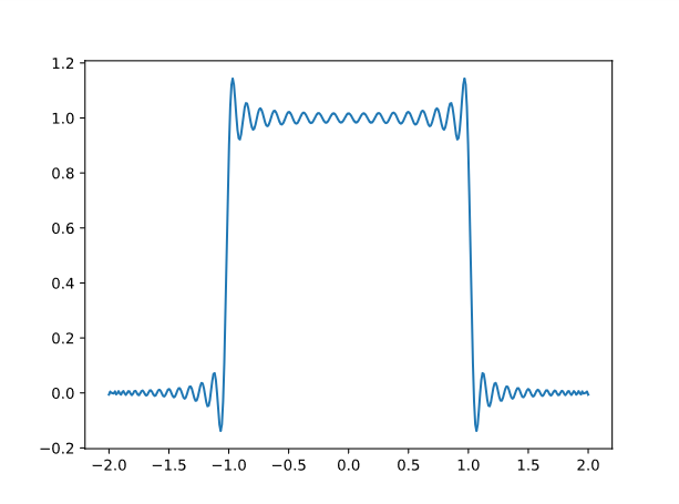
What if the function we’re interpolating isn’t smooth? If we consider the step function $f(x) = 1$ if $x\in[-1,1]$ and $f(x)=0$ elsewhere, show that the polynomial interpolation has Gibbs phenomena.
In the previous examples, we note that the approximation is very poor towards to the two ends where the error $R_n(x)=f(x)-P_n(x)$ is disappointingly high. This is known as Runge's phenomenon, indicating the fact that higher degree polynomial interpolation does not necessarily always produce more accurate result, as the degree of the interpolating polynomial may become unnecessarily high and the polynomial may become oscillatory. This Runge's phenomenon is a typical example of overfitting, due to an excessively complex model with too many parameters relative to the observed data, here specifically a polynomial of a degree too high (requiring too many coefficients) to model the given data points.
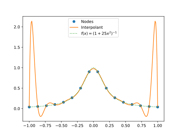 The smooth blue line is $f(x)$ and the wiggly orange line is $P_9(x)$.
Runge showed that polynomial interpolation at evenly-spaced points can fail spectacularly to converge.
In the following example we use the function $f(x) = \frac{1}{(1 + 25x^2)}$ on the interval $[-1, 1]$. Here we have $16$ interpolation nodes.
Runge found that in order for interpolation at evenly spaced nodes in $[-1, 1]$ to converge,
the function being interpolated needs to be analytic inside a "football-shaped" region of the complex plane
with major axis $[-1, 1]$ on the real axis and minor axis approximately $[-0.5255, 0.5255]$ on the imaginary axis.
The smooth blue line is $f(x)$ and the wiggly orange line is $P_9(x)$.
Runge showed that polynomial interpolation at evenly-spaced points can fail spectacularly to converge.
In the following example we use the function $f(x) = \frac{1}{(1 + 25x^2)}$ on the interval $[-1, 1]$. Here we have $16$ interpolation nodes.
Runge found that in order for interpolation at evenly spaced nodes in $[-1, 1]$ to converge,
the function being interpolated needs to be analytic inside a "football-shaped" region of the complex plane
with major axis $[-1, 1]$ on the real axis and minor axis approximately $[-0.5255, 0.5255]$ on the imaginary axis.
The function in Runge’s example has a singularity at $0.2i$, which is inside the "football region". Linear interpolation at evenly spaced points would converge for the function $f(x) = \dfrac{1}{(1 + x^2)}$ since the singularity is outside the "football region".
For smooth functions interpolating at more points does improve the fit if you interpolate at the roots of Chebyshev polynomials.
As you interpolate at the roots of higher and higher degree Chebyshev polynomials,
the interpolants converge to the function being interpolated. The plot below shows how interpolating at the roots of $T_{16}$,
the 16th Chebyshev polynomial, eliminates the bad behavior at the ends.
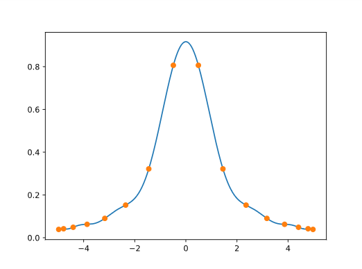
To make this plot, we replaced $x$ above with the roots of $T_{16}$, rescaled from the interval $[-1, 1]$ to the interval $[-5, 5]$ to match the example above.
                """ The chebychev abscissa """
                n = 16
                x = [np.cos(pi*(2*k-1)/(2*n)) for k in range(1, n+1)]
                x = 5*np.array(x)
Here’s the result of interpolating the indicator function of the interval $[-1, 1]$ at $100$ Chebyshev points. We get the same “bat ears” as before.
Sensibility of the interpolation polynomial solution to roundoff errors
We assume that the data $y_i$ are corrupted by a noise such that
$$ \hat{y}_i = y_i(1 + \epsilon_i)$$
where $|\epsilon_i| ≤ eps$ with $eps$ being the smallest number in the computer such that the rounded value of $1 + esp$ is greater than $1$.
We then want to study the difference between the polynomial solutions of $(x_i, y_i)$ and $(x_i, \hat{y}_i)$.
We have the following result.
Uniform data points case:
for $x_k=a+\dfrac{k}{n}(b-a)$ on $[a,b]$ we have $$ \Lambda_n(x) \underset{\infty}{\sim} \dfrac{2^{n+1}}{e.n.log(n)} $$
Chebyshev data points case:
for $x_k=\dfrac{a+b}{2}+\dfrac{b-a}{2}cos(\dfrac{(2k+1)\pi}{2n+2})$ we have $$ \Lambda_n(x) \underset{\infty}{\sim} \dfrac{2}{\pi}log(n) $$
Exercice [M-3]
Let $f(x)=sin(x)$ be defined on $[0,5]$.-
For any subdivision of the interval, calculate a bounded value of $R_n$ (use the Interpolation Error Theorem), the interpolation error of this function by $P_n(x)$. Apply it for $n=50$.
-
If $n=50$, calculate the Lebesgue constant for a Chebychev subdivision on $[0,5]$. Draw the interpolation polynomial solution.
If $n=50$, calculate the Lebesgue constant for a uniform subdivision on $[0,5]$. Draw the interpolation polynomial solution to these data.
Exercice [M-4]
Let $x_0=-1,x_1=0$ and $x_2=1$ be subdivision of $[-1,1]$.-
Draw the associated Lebesgue constant $\Lambda_2(x)$.
-
Show that for $x\in\ [x_{j-1},x_j]$ we have: $$ \Lambda_n(x) = \sum_{i=0}^{n} \delta_i L_i^n(x) $$ where $\delta_i = (-1)^{j-i+1}$ if $i \leq j-1$ and $\delta_i = (-1)^{i-j}$ if $i \geq j$
-
Show that $\Lambda_n(x)$ has a unique local maximum on each interval $[x_{j-1},x_j]$. For this, you can study the extrema of the $L_i^n(x)$.
Cubic Spline Interpolation
All previously discussed methods of polynomial interpolation fit a set of $n+1$ given points $y_i=f(x_i),\;(i=0,\cdots,n)$ by an $n$-th degree polynomial, and a higher degree polynomial is needed to fit a larger set of data points. A major drawback of such methods is overfitting, as demonstrated in the previous exercice.
Now we consider a different method of spline interpolation, which fits the given points by a piecewise polynomial function $S(x)$, known as the spline, a composite function formed by $n$ low-degree polynomials $P_i(x)$ each fitting $f(x)$ in the interval between $x_{i-1}$ and $x_i,\;(i=1,\cdots,n)$: $$ \displaystyle S(x)=\left\{ \begin{array}{cc} P_1(x) & x_0\le x\le x_1\\ \vdots & \vdots \\ P_i(x) & x_{i-1} \le x_i\\ \vdots & \vdots\\ P_n(x) & x_{n-1}\le x\le x_n \end{array}\right. $$ As this method does not use a single polynomial of degree $n$ to fit all $n+1$ points at once, it avoids high degree polynomials and thereby the potential problem of overfitting. These low-degree polynomials need to be such that the spline $S(x)$ they form is not only continuous but also smooth.
-
For $S(x)$ to be continuous, two consecutive polynomials $P_i(x)$ and $P_{i+1}(x)$ must join at $x_i$: $$ P_i(x_i)=P_{i+1}(x_i)=f(x_i)=y_i$$ Or, equivalently, $P_i(x)$ must pass the two end-points, i.e., $$ P_i(x_{i-1})=f(x_{i-1})=y_{i-1},\;\;\;\;\;P_i(x_i)=f(x_i)=y_i$$
-
For $S(x)$ to be smooth, they need to have the same derivatives at the point they joint, i.e., $$ P_i^{(k)}(x_i)=P_{i+1}^{(k)}(x_i)$$ must hold for some order $k$. The higher the order $k$ is, the more smooth the spline $S(x)$ becomes.
-
Linear spline: $P_i(x)=a_ix+b_i$ with two parameters $a_i$ and $b_i$ can only satisfy the following two equations required for $S(x)$ to be continuous: $$ P_i(x_i)=a_ix_i+b_i=f(x_i)=y_i,\;\;\;\;\;\;\;\; P_i(x_{i-1})=a_ix_{i-1}+b_i=f(x_{i-1})=y_{i-1} $$ or, equivalently, $P_i(x)$ has to pass the two end points $(x_{i-1},\,y_{i-1})$ and $(x_i,\,y_i)$: $$ \frac{P_i(x)-y_{i-1}}{x-x_{i-1}}=\frac{y_i-y_{i-1}}{x_i-x_{i-1}} $$ Solving either of two problems above, we get: $$ P_i(x)= a_ix+b_i =\frac{y_i-y_{i-1}}{h_i}\,x+\frac{x_iy_{i-1}-x_{i-1}y_i}{h_i} $$ and $$ P_i(x) = \frac{x-x_{i-1}}{h_i}y_i+\frac{x_i-x}{h_i}y_{i-1},\;\;\;\;\;\;\;\;\;\; (h_i=x_i-x_{i-1}) $$ which is represented in the form of $P_i(x)=a_ix+b_i$ by the first expression, or a linear interpolation of the two end points $y_{i-1}=f(x_{i-1})$ and $y_i=f(x_i)$ in the second expression. As $P_i(x_i)=P_{i+1}(x_i)=y_i$, the linear spline $S(x)$ is continuous at $x_i$. But as in general $$ P'_i(x_i)=\frac{y_i-y_{i-1}}{h_i}\ne P'_{i+1}(x_i)=\frac{y_{i+1}-y_i}{h_i} $$ $S(x)$ is not smooth, i.e., $k=0$.
-
Quadratic spline: $Q_i(x)=a_ix^2+b_ix+c_i$ with three parameters $a_i,\;b_i$ and $c_i$ can satisfy the following three equations required for $S(x)$ to be smooth ($k=1$) as well as continuous: $$ Q_i(x_i)=y_i,\;\;\;\;Q_i(x_{i-1})=y_{i-1},\;\;\;\;Q'_i(x_i)=Q'_{i+1}(x_i) $$ To obtain the three parameters $a_i$, $b_i$ and $c_i$ in $Q_i(x)$, we consider $Q'_i(x)=2a_ix+b_i$, which, as a linear function, can be linearly fit by the two end points $f'(x_{i-1})=D_{i-1}$ and $f'(x_i)=D_i$: $$ Q'_i(x)=\frac{x-x_{i-1}}{h_i}D_i+\frac{x_i-x}{h_i}D_{i-1} $$ Integrating, we get $$ Q_i(x)=\int Q'_i(x)\,dx=\frac{D_i}{2h_i}(x-x_{i-1})^2 -\frac{D_{i-1}}{2h_i}(x_i-x)^2+c_i $$ As $Q_i(x_i)=y_i$, we have $$ Q_i(x_i)=\frac{D_i}{2h_i}(x_i-x_{i-1})^2+c_i=\frac{D_ih_i}{2}+c_i=y_i $$ Solving this for $c_i$ $$ c_i=y_i-\frac{D_ih_i}{2} $$ and substituting it back into the expression of $Q_i(x)$, we get $$ Q_i(x)=\frac{D_i}{2h_i}(x-x_{i-1})^2-\frac{D_{i-1}}{2h_i}(x_i-x)^2 +y_i-\frac{D_ih_i}{2} $$ Also, as $Q_i(x_{i-1})=y_{i-1}$, we have $$ Q_i(x_{i-1})=-\frac{D_{i-1}h_i}{2}+y_i-\frac{D_ih_i}{2}=y_{i-1} $$ or $$ D_i=2\frac{y_i-y_{i-1}}{h_i}-D_{i-1},\;\;\;\;\;\;(i=1,\cdots,n) $$ Given $f'(x_0)=D_0$, we can get iteratively all subsequent $D_1,\cdots,D_n$ and thereby $Q_i(x)$. Alternatively, given $f'(x_n)=D_n$, we can also get iteratively all previous $D_{n-1},\cdots,D_0$. It is obvious that with only three free parameters, the quadratic polynomials cannot satisfy both boundary conditions $Q'_1(x_0)=f'(x_0)$ and $Q'_n(x_n)=f'(x_n)$.
-
Cubic spline: $C_i(x)=a_ix^3+b_ix^2+c_ix+d_i$ with four parameters $a_i,\;b_i,\;c_i$, and $d_i$ can satisfy the following four equations required for $S(x)$ to be continuous and smooth ($k=2$): $$ C_i(x_i)=y_i,\;\;\;\;C_i(x_{i-1})=y_{i-1},\;\;\;\; C'_i(x_i)=C'_{i+1}(x_i),\;\;\;\;\;\; $$ and $C''_i(x_i)=C''_{i+1}(x_i)$. To obtain the four parameters $a_i$, $b_i$, $c_i$ and $d_i$ in $C_i(x)$, we first consider $C''_i(x)=(a_ix^3+b_ix^2+c_ix+d_i)''=6a_ix+2b_i$, which, as a linear function, can be linearly fit by the two end points $f''(x_{i-1})=M_{i-1}$ and $f''(x_i)=M_i$: $$ C''_i(x)=\frac{x_i-x}{h_i} M_{i-1}+\frac{x-x_{i-1}}{h_i} M_i $$ Integrating $C''_i(x)$ twice we get $$ C_i(x)=\int\left(\int C''_i(x)\,dx\right)\;dx =\frac{(x_i-x)^3}{6h_i}M_{i-1}+\frac{(x-x_{i-1})^3}{6h_i}M_i+c_ix+d_i $$ As $C_i(x_{i-1})=y_{i-1}$ and $C_i(x_i)=y_i$, we have: $$ C_i(x_{i-1})=\frac{h_i^2}{6}M_{i-1}+c_ix_{i-1}+d_i=y_{i-1},\;\;\;\;\;\;\;\; C_i(x_i)=\frac{h_i^2}{6}M_i+c_ix_i+d_i=y_i $$ Solving these two equations we get the two coefficients $c_i$ and $d_i$: $$ c_i=\frac{y_i-y_{i-1}}{h_i}-\frac{h_i}{6}(M_i-M_{i-1}) $$ $$ d_i=\frac{x_iy_{i-1}-x_{i-1}y_i}{h_i}-\frac{h_i}{6}(x_iM_{i-1}-x_{i-1}M_i) $$ Substituting them back into $C_i(x)$ and rearranging the terms we get $$ C_i(x) = \frac{(x_i-x)^3}{6h_i}M_{i-1}+\frac{(x-x_{i-1})^3}{6h_i}M_i +\left(\frac{y_i-y_{i-1}}{h_i}-\frac{h_i}{6}(M_i-M_{i-1})\right)x $$ $$ +\frac{x_iy_{i-1}-x_{i-1}y_i}{h_i}-\frac{h_i}{6}(x_iM_{i-1}-x_{i-1}M_i) $$ $$ =\frac{(x_i-x)^3}{6h_i}M_{i-1}+\frac{(x-x_{i-1})^3}{6h_i}M_i +\left(\frac{y_{i-1}}{h_i}-\frac{M_{i-1}h_i}{6}\right) (x_i-x) +\left(\frac{y_i}{h_i}-\frac{M_ih_i}{6}\right) (x-x_{i-1}) $$ To find $M_i$ $(i=1,\cdots,n-1)$, we take derivative of $C_i(x)$ and rearrange terms to get $$ C'_i(x) = -\frac{(x_i-x)^2}{2h_i}M_{i-1}+\frac{(x-x_{i-1})^2}{2h_i}M_i -\frac{1}{h_i}(y_{i-1}-\frac{M_{i-1}h_i^2}{6}) +\frac{1}{h_i}(y_i-\frac{M_ih_i^2}{6}) $$ $$ C'_i(x) = -\frac{(x_i-x)^2}{2h_i}M_{i-1}+\frac{(x-x_{i-1})^2}{2h_i}M_i +\frac{y_i-y_{i-1}}{h_i}-\frac{h_i}{6}(M_i-M_{i-1}) $$ which, when evaluated at $x=x_i$ and $x=x_{i-1}$, becomes: $$ C'_i(x_i)$ = \frac{h_i}{3}M_i+\frac{y_i-y_{i-1}}{h_i}+\frac{h_i}{6}M_{i-1} =\frac{h_i}{6}(2M_i+M_{i-1})+f[x_{i-1},x_i] $$ $$ C'_i(x_{i-1}) = -\frac{h_i}{3}M_{i-1}+\frac{y_i-y_{i-1}}{h_i}-\frac{h_i}{6}M_i =-\frac{h_i}{6}(2M_{i-1}-M_i)+f[x_{i-1},x_i] $$ Replacing $i$ by $i+1$ in the second equation, we also get $$ C'_{i+1}(x_i)=-\frac{h_{i+1}}{3}M_i+\frac{y_{i+1}-y_i}{h_{i+1}} -\frac{h_{i+1}}{6}M_{i+1} $$ To satisfy $C'_i(x_i)=C'_{i+1}(x_i)$, we equate the above to the first equation to get: $$ \frac{h_i}{3}M_i+\frac{y_i-y_{i-1}}{h_i}+\frac{h_i}{6}M_{i-1} =-\frac{h_{i+1}}{3}M_i+\frac{y_{i+1}-y_i}{h_{i+1}}-\frac{h_{i+1}}{6}M_{i+1} $$ Multiplying both sides by $6/(h_{i+1}+h_i)=6/(x_{i+1}-x_{i-1})$ and rearranging, we get: $$ \frac{h_i}{h_{i+1}+h_i}M_{i-1}+2M_i+\frac{h_{i+1}}{h_{i+1}+h_i}M_{i+1}=6f[x_{i-1},x_i,x_{i+1}] $$ Note that here $$ \frac{1}{x_{i+1}-x_{i-1}}\left(\frac{y_{i+1}-y_i}{x_{i+1}-x_i}\right) =\frac{f[x_i,x_{i+1}]-f[x_{i-1},x_i]}{x_i-x_{i-1}} =f[x_{i-1},x_i,x_{i+1}] $$ is simply the second divided differences. We can rewrite the equation above as $$ \mu_iM_{i-1}+2M_i+\lambda_iM_{i+1}=6\,f[x_{i-1},x_i,x_{i+1}],\;\;\;\;\;\;\;(i=1,\cdots,n-1) $$ where $$ \mu_i=\frac{h_i}{h_{i+1}+h_i},\;\;\;\; \lambda_i=\frac{h_{i+1}}{h_{i+1}+h_i}=1-\mu_i $$ Here we have $n-1$ equations but $n+1$ unknowns $M_0,\cdots,M_n$. To obtain these unknowns, we need to get two additional equations based on certain assumed boundary conditions. Assume the first order derivatives at both ends $f'(x_0)$ and $f'(x_n)$ are known. Specially $f'(x_0)=f'(x_n)=0$ is called clamped boundary condition. At the front end, we set $$ C'_1(x_0)=-\frac{h_1}{3}M_0+\frac{y_1-y_0}{h_1}-\frac{h_1}{6}M_1 =-\frac{h_1}{3}M_0-\frac{h_1}{6}M_1+f[x_0,x_1]=f'(x_0) $$ Multiplying $-6/h_1=-6/(x_1-x_0)$ we get $$ 2M_0+M_1=\frac{6}{x_1-x_0}[f[x_0,x_1]-f'(x_0)]=6\,f[x_0,x_0,x_1] $$ Similarly, at the back end, we also set $$ C'_n(x_{n})=\frac{h_n}{3}M_n+\frac{y_n-y_{n-1}}{h_n} +\frac{h_n}{6}M_{n-1} =\frac{h_n}{3}M_n+\frac{h_n}{6}M_{n-1}+f[x_{n-1},x_n]=f'(x_n) $$ Multiplying $6/h_n=6/(x_n-x_{n-1})$ we get $$ 2M_n+M_{n-1}=\frac{6}{x_n-x_{n-1}}[f'(x_n)-f[x_{n-1},x_n]]=6\,f[x_{n-1},x_n,x_n] $$ We can combine these equations into a linear equation system of $n+1$ equations and the same number of unknowns: $$ \left[ \begin{array}{ccccc} 2 & 1 & & & \\ \mu_1 & 2 & \lambda_1 \\ \vdots \\ ...,x_2]\\ \vdots\\ f[x_{n-2},x_{n-1},x_n]\\ f[x_{n-1},x_n,x_n] \end{array}\right] $$ Alternatively, we can also assume $f''(x_0)$ and $f''(x_n)$ are known. Specially $f''(x_0)=f''(x_n)=0$ is called natural boundary condition. Now we can simply get $M_0=f''(x_0)$ and $M_n=f''(x_n)$ and solve the following system for the $n+1$ unknowns $M_0,\cdots,M_n$: $$ \left[ \begin{array}{ccccc} 1 & 0 & & & \\ \mu_1 & 2 & \lambda_1 ...f[x_0,x_1,x_2]\\ \vdots\\ 6f[x_{n-2},x_{n-1},x_n]\\ f''(x_n) \end{array}\right] $$
Exercice [PY-4]
In this exercice, we want to calculate the polyomial spline interpolation to the runge function.-
Define the LinearSpline(x,X,Y), QuadraticSpline(x,X,Y) and CubicSpline(x,X,Y) functions.
Apply these functions for the interpolation of uniform data of the runge function. Draw the resulting curves.
References
- J.H. Ahlberg, E.N. Nilson & J.L. Walsh (1967) The Theory of Splines and Their Applications. Academic Press, New York.
- C. de Boor (1978) A Practical Guide to Splines. Springer-Verlag.
- G.D. Knott (2000) Interpolating Cubic Splines. Birkhäuser.
- H.J. Nussbaumer (1981) Fast Fourier Transform and Convolution Algorithms. Springer-Verlag.
- H. Späth (1995) One Dimensional Spline Interpolation. AK Peters.