Linear Least Squares Fitting

Introduction

We are likely all familiar with the concept of curve-fitting — sometimes, we, as humans, can recognize certain patterns in data about which the data itself is agnostic. If we look at a chart like the following: We think immediately of a linear relationship. But what tools can we use to precisely determine a line from these individual points of data? Intuitively speaking, we can all figure this out pretty easily — we want to find the line that is minimally far from every single one of these points. The way this is actually implemented is through a method known as least squares regression. This form of regression is very powerful, and is widely used in applications from signals processing to economics research. Least squares fitting finds the best curve to fit a set of points through minimizing the sum of the squares of the offsets of each point from the curve.

Linear Regression

Suppose that we have measured three data points ${\cal P}=\left\{(-1,3),(1,1),(2,2)\right\}$, and that our model for these data asserts that the points should lie on a line. Of course, these three points do not actually lie on a single line, but this could be due to errors in our measurement. How do we predict which line they are supposed to lie on?

The general equation for a (non-vertical) line is $y=a_0+a_1x$. If our three data points were to lie on this line, then the following equations would be satisfied: \[ \left\{ \begin{array}[c]{l} a_{0}-a_{1}=3\\ a_{0}+a_{1}=1\\ a_{0}+2a_{1}=2 \end{array} \right. \] In order to find the best-fit line, we try to solve the above equations in the unknowns $a_0$ and $a_1$. Putting our linear equations into matrix form, we are trying to solve ${\bf A x}={\bf b}$ where \[ {\bf A}=\left( \begin{array}[c]{cc} 1 & -1\\ 1 & 1\\ 1 & 2 \end{array} \right) \;\;\;\; {\bf x}=\left( \begin{array}[c]{c} a_0 \\ a_1\\ \end{array} \right) \;\;\;\; {\bf b}=\left( \begin{array}[c]{c} 3 \\ 1\\ 2 \end{array} \right) \] As the three points do not actually lie on a line, there is no actual solution. So instead we have to compute an approximate solution.

Consequently, we have to answer to the following important question:
Suppose that ${\bf A x}={\bf b}$ does not have a solution. What is the best approximate solution?

For our purposes, the best approximate solution is called the least-squares solution. Least squares fitting finds the best curve to fit a set of points through minimizing the sum of the squares of the offsets of each point from the curve. We use the squares of the offsets to ensure the differentiability property, which allows us to linear tools from calculus in analyzing the data. We will present two methods for finding least-squares solutions, and we will give several applications to best-fit problems. We begin by clarifying exactly what we will mean by a “best approximate solution” to an inconsistent matrix equation ${\bf A x}={\bf b}$.

The term “least squares” comes from the fact that $\left\| {\bf A.x} - {\bf b} \right\|_2$ is the square root of the sum of the squares of the entries of the vector ${\bf A.x} - {\bf b}$. So a least-squares solution minimizes the sum of the squares of the differences between the entries of ${\bf A x}$ and ${\bf b}$. In other words, a least-squares solution solves the equation ${\bf A x}={\bf b}$ as closely as possible, in the sense that the sum of the squares of the difference ${\bf A.x} - {\bf b}$ is minimized.

Example: Let $y=a_0+a_1x$ be a linear model of the data ${\cal P}=\{ (0,\,1),\;(2,\,1.9),\;(4,\,3.2) \}$. Then we have to solve the overdetermined linear system ${\bf A x}={\bf b}$ by using a least squares solution where \begin{equation} {\bf A}^T=\left[\begin{array}{ccc}1&1&1\\0&2&4\end{array}\right], \;\;\;\;\;{\bf b}^T=[1,\,1.9,\,3.2] \end{equation} As the rank of the matrix is equal to $2$, by using the previous Theorem, it yields: \begin{equation} \hat{{\bf x}}={\bf A}^+ {\bf b}=({\bf A}^T{\bf A})^{-1}{\bf A}^T\;{\bf b} =[0.93,\,0.55]^T \end{equation} Consequently, $y=0.93+0.55x$ is the unique least squares solution to this problem.

You may have noticed that we have been careful to say “the least-squares solutions” in the plural, and “a least-squares solution” using the indefinite article. This is because a least-squares solution need not be unique: indeed, if the columns of ${\bf A}$ are linearly dependent, then the least-squares solution of ${\bf A x}={\bf b}$ has infinitely many solutions. The previous theorem, gives us a criteria for uniqueness.

Exercice [PY-1]

• We wish to calculate the least-square approximation of the previous data ${\cal P}=\left\{ (-1,3),(1,1),(2,2) \right\}$ with a polynomial function of degree $n=1$.
  Firstly, write this problem as an interpolation problem of the form $\mathbf{A}.\mathbf{x}=\mathbf{b}$. We then obtain an overdetermined system. We propose to solve it by minimizing the following function: $$ \underset{\left(a_{0},a_{1}\right)\in\mathbb{R}^2}{\min}F\left(a_{0},a_{1}\right)=||\mathbf{A}.\mathbf{x}-\mathbf{b}||^{2} $$ Show that $$ ||\mathbf{A}.\mathbf{x}-\mathbf{b}||^{2}=\sum_{j=1}^{3}\left(a_0+a_1x_{j}-y_{j}\right)^{2} $$

• By writting all the partial derivatives of $F$ and by solving $\dfrac{\partial F}{\partial a_{0}}=0$ and $\dfrac{\partial F}{\partial a_{1}}=0$ show that we have to solve $\mathbf{A}^{T}\mathbf{A}.\mathbf{x}=\mathbf{A}^{T}{\bf b}$.

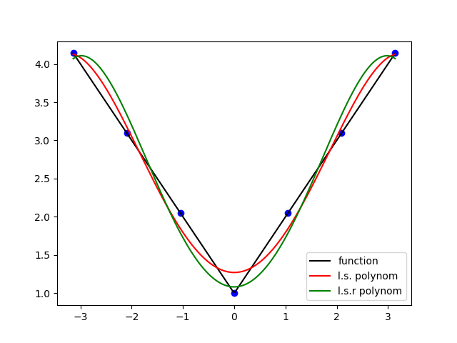
• Draw the data points and the linear function solution to this system.



Let $f(x) = \cos(x)$ be a real function defined on $[0,2\pi]$.
We select $p=10$ or $p=20$ uniform data points on this interval $$ {\cal P}=\left\{ \left( x_j=\frac{(j-1)}{p}\pi,y_j=f(x_j) \right) \;\;\; {\text for }\;\; j=1,...,p \right\} $$
• Calculate the best least-squares polynomial approximation $P_4(x)=a_0+a_1x+a_2x^2+a_3x^3+a_4x^4$ of degree equal or less than $n=4$ of these data points ${\cal P}$.
• Print the maximum error.

• Draw the data points and the polynomial solution $P_4(x)$.

• In this part we want to minimize the sum of the squares of the relative errors: $$ \varepsilon_j = \frac{P_4\left( x_{j}\right) - y_{j} }{y_{j} } $$ For this we want to minimize the following function: \begin{align*} F\left(a_{0},a_{1},\ldots,a_{4}\right) & = \sum_{j=1}^{p} \varepsilon_j^{2}\\ & =\sum_{j=1}^{p} w_{j}\left( P_4\left( x_{j}\right) - y_j \right) ^{2} \end{align*} where the values $w_{j}=\dfrac{1}{\left( y_{j} \right) ^{2}}$ are called the weights of the data points. We assume that $y_j \neq 0$. Consequently, the data with high values $y_j$ are less sensitive in the minimization process.
  Show that, in this case, we have to solve the following linear system: $$ {\bf A}^{T}.{\bf W}.{\bf A}.{\bf x}={\bf A}^{T}.{\bf W}.{\bf b} $$ where ${\bf W}$ is a $p \times p$ diagonal matrix with the $w_j$ as diagonal values.

import numpy as np
import matplotlib.pyplot as plt
import numpy.linalg as LA

print("*******************") 
print("PY-1")
print("*******************") 



# création de la liste des données à interpoler
def f(x):
    return np.abs(x)+1

# Horner Algorithm
def Horner(x,coeff):
    p=len(coeff)
    s=coeff[p-1]
    for i in range(p-1):
        s=x*s+coeff[p-2-i]
    return s

# nombre de points
p=7
# degré du polynôme
n=4
# intervalle
a=-np.pi
b= np.pi

X=np.linspace(a,b,p)
Y=f(X)

# Création de la matrice d'interpolation
A=np.zeros((p,n+1))

for i in range(p):
    for j in range(n+1):
        A[i,j]=X[i]**j
        
#print("matrice interpolation: ")
#print(np.round(A,1))
# résolution
coeff=LA.solve(np.dot(np.transpose(A),A),np.dot(np.transpose(A),Y))
#print("mat= ",np.dot(np.transpose(A),A)," b= ",np.dot(np.transpose(A),Y))
print("solution= ",coeff)

err1 = [np.abs(Horner(X[i],coeff)-Y[i]) for i in range(p)]
print("\nmax error data points = ",np.max(err1))

t=np.linspace(a,b,200)
err2 = [np.abs(Horner(t[i],coeff)-f(t[i])) for i in range(len(t))]
print("\nmax error data |polynom -function| = ",np.max(err2))

print("\nRelative error minimization")

w = [1/Y[i]**2 for i in range(p)]
W = np.diag(w)

# résolution
coeffr=LA.solve(np.dot(np.transpose(A),np.dot(W,A)),np.dot(np.transpose(A),np.dot(W,Y)))
print("solution= ",coeffr)
err1 = [np.abs(Horner(X[i],coeffr)-Y[i]) for i in range(p)]
print("\nmax error data points = ",np.max(err1))

t=np.linspace(a,b,200)
err2 = [np.abs(Horner(t[i],coeffr)-f(t[i])) for i in range(len(t))]
print("\nmax error data |polynom -function| = ",np.max(err2))

plt.clf()
p1=plt.plot(X,Y,'bo')
p2=plt.plot(t,f(t),'k',label='function')
p3=plt.plot(t,Horner(t,x),'r',label="l.s. polynom")
p3=plt.plot(t,Horner(t,xr),'g',label="l.s.r polynom")
plt.legend(loc='lower right')
plt.show()
plt.savefig('PY1.png')

Exercice [PY-2]

Gauss invented the method of least squares to find a best-fit ellipse: he correctly predicted the (elliptical) orbit of the asteroid Ceres as it passed behind the sun in 1801.

• Find the best least square ellipse through the points ${\cal P}=\left\{(0,2),(2,1),(1,−1),(−1,−2),(−3,1),(−1,−1) \right\}$. What quantity is being minimized?

• Solve this problem with the numpy python library and draw the best least-squares ellipse solution. For this, you can use the contour function of matplotlib.pyplot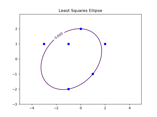

  

print("\n***************")
print("Exercice PY-2")
print("***************\n")

def ellipse(x,y,c):
    res = x*x+c[0]*y*y+c[1]*x*y+c[2]*x+c[3]*y+c[4]
    return res

P=[[0,2],[2,1],[1,-1],[-1,-2],[-3,1],[-1,1]]
xp = np.transpose(P)[0]
yp = np.transpose(P)[1]  

# Approximation au sens des moindres carrées de la conique
A=[]
b=[]
for i in range(len(P)):
    x=P[i][0]
    y=P[i][1]
    A.append([y*y,x*y,x,y,1])
    b.append(-x*x)
coeff=LA.solve(np.dot(np.transpose(A),A),np.dot(np.transpose(A),b))

#calcul de la grille des valeurs et de la conique
delta = 0.025
x = np.arange(-5.0, 5.0, delta)
y = np.arange(-3.0, 3.0, delta)
X, Y = np.meshgrid(x, y)
Z=ellipse(X,Y,coeff)


plt.clf()
#tracé des points
p1=plt.plot(xp,yp,'bo')
CS=plt.contour(X, Y, Z,levels = np.arange(0.0, 1.0, 5.0),extend='both')
plt.clabel(CS,inline=1,fontsize=10)
plt.title("Least Squares Ellipse")
plt.savefig('ellipse.png')

Segmented Linear Regression

Segmented linear regression (SLR) addresses this issue by offering piecewise linear approximation of a given dataset [2]. It splits the dataset into a list of subsets with adjacent ranges and then for each range finds linear regression, which normally has much better accuracy than one line regression for the whole dataset. It offers an approximation of the dataset by a sequence of line segments. In this context, segmented linear regression can be viewed as a decomposition of a given large dataset into a relatively small set of simple objects that provide compact but approximate representation of the given dataset within a specified accuracy. Segmented linear regression provides quite robust approximation. This strength comes from the fact that linear regression does not impose constraints on ends of a line segment. For this reason, in segmented linear regression, two consecutive line segments normally do not have a common end point. This property is important for practical applications, since it enables us to analyse discontinuities in temporal data: sharp and sudden changes in the magnitude of a signal, switching between quasi-stable states. This method allows us to understand the dynamics of a system or an effect. For comparison, high degree polynomial regression provides a continuous approximation [3]. Its interpolation and extrapolation suffer from overfitting oscillations [4]. Polynomial regression is not a reliable predictor in applications mentioned earlier. Despite the simple idea, segmented linear regression is not a trivial algorithm when it comes to its implementation. Unlike linear regression, the number of segments in an acceptable approximation is unknown. The specification of the number of segments is not a practical option, since a blind choice produces usually a result that badly represents a given dataset. Similarly, uniform splitting a given dataset into equal-sized subsets is not effective for achieving an optimal approximation result. Instead of these options, we place the restriction of the allowed deviation and attempt to construct an approximation that guarantees the required accuracy with as few line segments as possible. The line segments detected by the algorithm reveal essential features of a given dataset. The deviation at a specified x value is defined as the absolute difference between original and approximation y values. The accuracy of linear regression in a range and the approximation error are defined as the maximum of all of the values of the deviations in the range. The maximum allowed deviation (tolerance) is an important user interface parameter of the model. It controls the total number and lengths of segments in a computed segmented linear regression. If input value of this parameter is very large, there is no splitting of a given dataset. The result is just one line segment of linear regression. If input value is very small, then the result may have many short segments. It is interesting to note that within this formulation, the problem of segmented linear regression is similar to the problem of polyline simplification. The solution to this problem provides the algorithm of Ramer, Douglas and Peucker [5]. Nevertheless, there are important reasons why polyline simplification is not the best choice for noisy data. This algorithm gives first priority to data points the most distant from already constructed approximation line segments. In the context of this algorithm, such data points are the most significant. The issue is that in the presence of noise, the significant points normally arise from high frequency fluctuations. The biggest damage is caused by outliers. For this reason, noise can have substantial effect on the accuracy of polyline simplification. In piecewise linear regression, each line segment is balanced against the effect of noise. The short term fluctuations are removed to show significant long term features and trends in original data.

Linear Approximation Theory: an introduction

Approximation theory is concerned with the ability to approximate functions by simpler and more easily calculated functions. The first question we ask in approximation theory concerns the possibility of approximation. Is the given family of functions from which we plan to approximate dense in the set of functions we wish to approximate? In this section we survey some of the main density results and density methods.

Let us consider the following function $f(x)=|x|$, we want to find a polynom function $P_n(x)$ of degree $n$ which closely approximates $f$. One way to choose this polynom is to minimized the "area" or the "distance" between $f$ and $P_n$.

Let $E=C^{0}\left( \left[ a,b\right] \right) $ be the vector space of continuous functions on $\left[ a,b\right] $ (with $a\lt b$) into $\mathbb{R}$. We can easily show that the polynomial vector space $\cal{P}_n$ belongs to $C^{0}\left( \left[ a,b\right] \right) $.

• $w(x)=1$ or $w(x)=\dfrac{1}{\sqrt{1-x^2}}$ on $]-1,1[$
• $w(x)=e^{-x^2}$ on $]-\infty,\infty[$

Exercice [M-1]

• Show that for any $f\in E$, $ \left\| f\right\| _{2}=\left( \int_{a}^{b} \left|f\left( x\right) \right| ^{2}dx\right) ^{\frac{1}{2}} $ is a norm.

• Show that $ \left\| f \right\| _{1} = \int_{a}^{b} \left| f\left( x\right) \right| dx $ is also a norm. Show that we cannot associate a scalar product to this norm.

• We set $a=0$ and $b=1$. We consider the following functions $f(x)=x^2$ and $P_\lambda(x)=\lambda x$ where $\lambda \in [0,1]$. Calculate the optimal values of $\lambda$ in the following minimization problems: $ \min_{\lambda\in [0,1]} \left\| f-P_\lambda \right\| _{1} \text{ and } \min_{\lambda\in [0,1]} \left\| f-P_\lambda \right\| _{2} $

This condition can be interpreted geometrically. Among all the polynoms $ Q_n$ of $\cal{P}_{n}$ the solution $P_n$ is obtained as the orthogonal projection of $f$ on the vector space $\cal{P}_n$ which is included in $E$.

Exercice [PY-3]

We want to calculate $P_2$, the best least square polynomial approximation of $f(x)=|x|$ on $[-1,1]$. For this, we consider the following scalar product: $\left\langle f,g\right\rangle =\int_{a}^{b} f\left(x\right) g\left( x\right) dx$.

• By using the necessary and sufficient condition, show that the solution $P_2(x)=a_0+a_1x+a_2x^2$ can be obtained by solving the following linear system: $$ \left[ \begin{array} [c]{ccc}% \left\langle 1,1 \right\rangle & \left\langle 1,x \right\rangle & \left\langle 1,x^2 \right\rangle\\ \left\langle x,1 \right\rangle & \left\langle x,x \right\rangle & \left\langle x,x^2 \right\rangle\\ \left\langle x^2,1 \right\rangle & \left\langle x^2,x \right\rangle & \left\langle x^2,x^2 \right\rangle\\ \end{array} \right] \left[ \begin{array}{c} a_0 \\ a_1 \\ a_2 \\ \end{array} \right] = \left[ \begin{array}{c} \left\langle f,1 \right\rangle \\ \left\langle f,x \right\rangle \\ \left\langle f,x^2 \right\rangle \\ \end{array} \right] $$

• Calculate all the coefficients of the previous system and solve it with python.

• Draw the function and polynom $P_2$.

• If the scalar product becomes $\left\langle f,g\right\rangle =\int_{a}^{b}w\left( x\right) f\left( x\right) g\left( x\right) dx$ then the we have to solve the following system: \[ \underset{j=0}{\overset{p}{\sum}}\left( \int_{-1}^{1}w\left( x\right) x^{j+k}dx\right) a_{j}=\int_{-1}^{1}w\left( x\right) f\left( x\right) x^{k}dx \] Calculate the new solution when $w(x)=\dfrac{1}{\sqrt {1-x^2}}$ on $]-1,1[$.

        
import numpy as np
import time
from numpy import linalg as LA
import matplotlib.pyplot as plt


def f(x):
    return np.abs(x)

def Pol(x,coeff):
    s = 0.0
    # TO DO
    return s

# Define the matrix
def Mat(X):
    n=len(X)-1
    A=np.zeros((n+1,n+1))
    # TO DO
    return A

# degree of the polynom
n=2

#Plot function f
t=np.linspace(a,b,100)
p2=plt.plot(t,f(t),'k')

#TO DO: solve the linear system

# Plot the polynom
p3=plt.plot(t,Pol(t,coeff),'r')
        
    

                        
import numpy as np
from numpy import linalg as LA
import matplotlib.pyplot as plt

# Interpolation polynomiale
print("Interpolation polynomiale")
def f(x):
    return np.abs(x)
    #return (x**2-4*x+4)*(x**2+4*x+2) 

# nombre de point d'interpolation
p=5
# degré du polynôme
n=p-1
# création de la liste des données à interpoler
a=-1.0
b= 1.0

# Horner Algorithm
def Pol(x,coeff):
    p=len(coeff)
    s=coeff[p-1]
    for i in range(p-1):
        s=x*s+coeff[p-2-i]
    return s


X=np.linspace(a,b,p)
Y=f(X)

t=np.linspace(a,b,1000)
plt.ylim(-1,2)
p1=plt.plot(X,Y,'bo')


# Création de la matrice d'interpolation
A=np.eye(n+1)
for i in range(n+1):
    for j in range(n+1):
        A[i,j]=X[i]**j    

# Resolution de AX=Y
coeff=LA.solve(A,Y)
print("coefficients = ",coeff)

p2=plt.plot(t,f(t),'k')
p3=plt.plot(t,Pol(t,coeff),'r')
plt.show()

References

- C. Eckart, G. Young, The approximation of one matrix by another of lower rank. Psychometrika, Volume 1, 1936, Pages 211–8. doi:10.1007/BF02288367
- C. de Boor (1978) A Practical Guide to Splines. Springer-Verlag.
- G.D. Knott (2000) Interpolating Cubic Splines. Birkhäuser.
- H.J. Nussbaumer (1981) Fast Fourier Transform and Convolution Algorithms. Springer-Verlag.
- H. Späth (1995) One Dimensional Spline Interpolation. AK Peters.