Image Compression

Introduction

In this study, we want to compress images by using two methods: JPEG and Singular Value Decompositon.
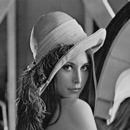
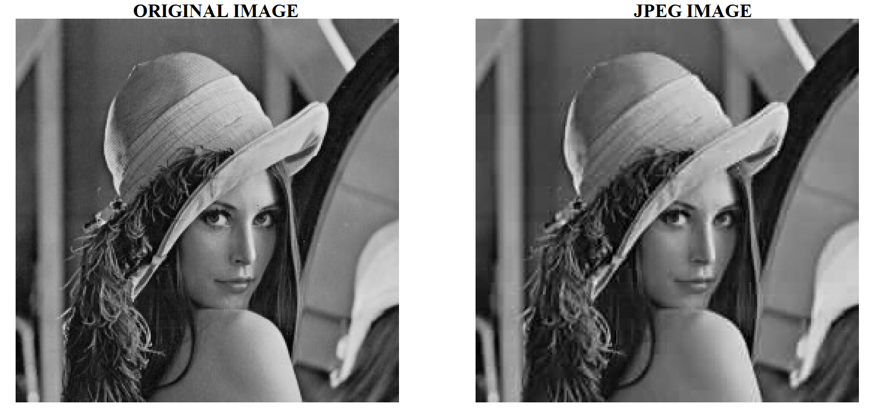
We assume that the images are grayscale images. Each pixel is represented by a brightness value ranging from $0$ (black) to $255$ (white) (respectively $0$ to $1$). A color image (or RGB image) can be easily converted to a grayscale image. In the following example, we will compress the lena.jpg (download it !) grayscale image. We first build a matrix ${\bf A}$ where the coordinates $(i, j)$ are the coordinates of the pixels of the image and the values $a_{ij}$ are the grayscale image values. Consequently, each pixel coordinates $(i,j)$ has an integer value $a_{ij}$ between $0$ and $255$ corresponding to the gray value of the pixel.

from math import*
from numpy.random import*
import random
import numpy as np
import scipy.linalg as sl
import matplotlib.image as mpimg
import matplotlib.pyplot as plt


A = mpimg.imread('lena.png')
A = A * 255

JPEG compression and Discrete Cosines Transform

Introduction

Every JPEG image is actually stored as a series of compressed image tiles that are usually only $8 \times 8$ pixels in size. The proper name for one of these tiles is the MCU or Minimum Coded Unit. When one refers to image blocking artifacts, they are really talking about visual discontinuities observed between one or more of these tiles. You can see the edges or boundaries of these tiles in JPEG images that have been compressed at a very low quality. The Minimum Coded Unit size for JPEG images is usually $8 \times 8$ pixels in size. For JPEG compression and decompression algorithms to work, an image must be represented by an integer number of complete MCUs. In other words, the X and Y dimensions typically need to be a multiple of $8$ pixels. The JPEG image compression standard is a lossy compression standard that uses the DCT transform and its associated properties to significantly reduce the number of bits used to represent an image. The encoding process involves many steps, which were broken down in our design as separable modules. After the transform, the top-left coefficient gives spacial DC information, while the bottom-right coefficient gives the highest spacial frequency (in both the horizontal and vertical direction) information. The spacial frequency representation is shown in the figure below.

1. Segmentation into Blocks

   The raw image data is chopped into 8x8 pixel blocks (these blocks are the Minimum Coded Unit). This means that the JPEG compression algorithm depends heavily on the position and alignment of these boundaries.

2. Discrete Cosine Transformation (DCT)

   The image is transformed from a spatial domain representation to a frequency domain representation. This is perhaps the most confusing of all steps in the process and hardest to explain. Basically, the contents of the image are converted into a mathematical representation that is essentially a sum of wave patterns.

3. Quantization

   Given the resulting wave equations from the DCT step, they are sorted in order of low-frequency components (changes that occur over a longer distance across the image block) to high-frequency components (changes that might occur every pixel). Is it widely known that humans are more critical of errors in the low-frequency information than the high-frequency information. The JPEG algorithm discards many of these high-frequency (noise-like) details and preserves the slowly-changing image information. This is done by dividing all equation coefficients by a corresponding value in a quantization table and then rounding the result to the nearest integer. Components that either had a small coefficient or a large divisor in the quantiziation table will likely round to zero. The lower the quality setting, the greater the divisor, causing a greater chance of a zero result. On the converse, the highest quality setting would have quantization table values of all 1's, meaning the all of the original DCT data is preserved.

4. Zigzag Scan

   The resulting matrix after quantization will contain many zeros. The lower the quality setting, the more zeros will exist in the matrix. By re-ordering the matrix from the top-left corner into a 64-element vector in a zig-zag pattern, the matrix is essentially sorted from low-frequency components to high-frequency components. As the high-frequency components are the most likley to round to zero, one will typically end up with a run of zeros at the end of the 64-entry vector. This is important for the next step.

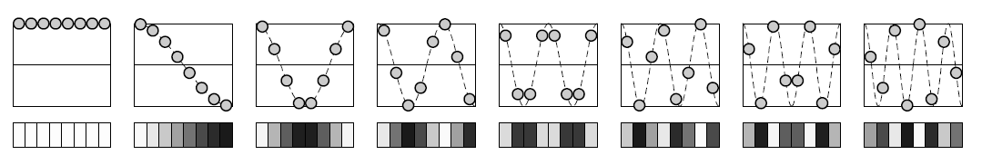
1D Fourier Serie and Discrete Cosines Transform

A Fourier series is an expansion of a $2\pi$-periodic function $f(x)$ (i.e. $f(x+2\pi)=f(x)$) in terms of an infinite sum of sines and cosines. Fourier series make use of the orthogonality relationships of the sine and cosine functions. The computation and study of Fourier series is extremely useful as a way to break up an arbitrary periodic function into a set of simple terms that can be plugged in, solved individually, and then recombined to obtain the solution to the original problem or an approximation to it to whatever accuracy is desired or practical. The computation of the Fourier series is based on the following integral identities discovered by Euler (1777, Opera vol 16, Pars I, p. 333).

Note that the coefficient of the constant term $a_0$ has been written such that to preserve symmetry with the definitions of $a_k$ and $b_k$.

For image compression, in general $f$ is not periodic. We cannot apply the Fourier series expansion. Nevertheless, we assume that $f(x)$ is a continuous function on $[0, \pi]$. We can extend this function by an even function $f(−x) = f(x)$. Consequently, it can be a 2$\pi$-periodic function. Consequently, the Fourier serie expansion only contains cosines terms:

we then have $a_k=\dfrac{2}{\pi} \int_{0}^{\pi}f(x) \cos(kx)dx$.
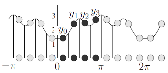
Let $x_j=\dfrac{(2j+1)\pi}{2N}$ for $j=0,...,N-1$ be uniform abscissa and $y_j=f(x_j)$ the values of function $f$ for the $x_j$. In the previous figure $N=4$.
If we replace $f(x_j)$ by $y_j$ in the previous cosine expansion and we bound the value of $k$ we obtain: $$ y_j = \dfrac{z_0}{2}+\sum_{k=1}^{N-1}z_k \cos(kx_j) $$ Consequently, the Discrete Cosines Transform values ($a_k \;\;\rightarrow \;\;z_k$) are defined by: $$ z_k = \dfrac{2}{N}\sum_{j=0}^{N-1}y_j \cos(kx_j) $$

2D Discrete Cosines Transform

We denote by $y_{i,j}$ the grayscale values of an image for each pixel $(i,j)$. We then have $$ y_{i,j} =\dfrac{2}{N} \sum_{k=0}^{N-1}\sum_{ℓ=1}^{N-1} c(k)c(ℓ) z_{k,ℓ} \cos(kx_i) \cos(ℓx_j) $$ where $c(k)=\dfrac{1}{\sqrt{2}}$ if $k=0$, $c(k)=1$ else,
and $$ z_{k,ℓ} = \dfrac{2c(k)c(ℓ)}{N} \sum_{i=0}^{N-1}\sum_{j=0}^{N-1}y_{i,j} \cos(kx_i)\cos(ℓx_j) $$

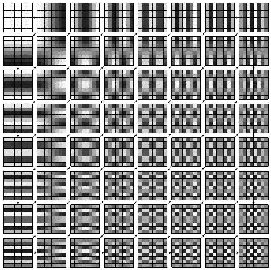
The use of this basis for image compression was introduced by Ahmed, Natarajan et Rao (IEEE 1974). To perform the first step of JPEG compression, the image in question is first split into $8 \times 8$ blocks of pixels. A 2-dimensional DCT is then applied to each $8 \times 8$ block. The results of a 2-D DCT represent the spacial frequency information of the original block at discrete frequencies corresponding to the index into the matrix. After the transform, the top-left coefficient gives spacial DC information, while the bottom-right coefficient gives the highest spacial frequency (in both the horizontal and vertical direction) information. The spacial frequency representation is shown in the figure above.

Notice the upper-left elements have lower spacial frequency both in the horizontal and vertical directions, while the lower-right elements have higher frequencies. With a DCT, most of the original information can be reconstructed from the lower frequency coefficients (the ones closer to the top-left), because of the high-energy compaction in those coefficients. Additionally, the human visual system is less perceptive to errors in high-frequency spacial content. These two facts together mean that errors in the low-frequency coefficients will be significantly more noticeable to human beings than errors in the high-frequency elements.

Quantization

Once the DCT is applied to the $8 \times 8$ block, a quantization factor is applied to the coefficients. This step, in short, discretizes the coefficients with step sizes related to the energy densities. Low-frequency coefficients are quantized with smaller step sizes, thus giving a smaller error than those quantized with larger step sizes. The low-frequency coefficients are quantized as such to reduce the likelihood of quantization errors. The higher frequencies are given larger step sizes thus reducing the accuracy in the less important elements. This is the lossy step in the compression process.

Though the JPEG compression standard does not specify a quantization matrix ${\bf Q}$ to use, this is one of the suggested matrices. To quantize the result of the 2-D DCT, each coefficient is divided by the appropriate value from the matrix above and rounded to the nearest integer. Coefficients $z_{k,ℓ}$ are then quantized. If their value are less than a given threshold they are set to zero. For example, for images with blue sky, only two or three coefficients will be different of zero which gives us a good compression factor.

Let’s go through an example. For each $z_{k,ℓ}$ coefficients of the DCT matrix we calculate the following quantized value: $$ z^*_{k,ℓ} = \dfrac{z_{k,ℓ}+Q_{k,l}}{Q_{k,l}} $$ If $|z^*_{k,ℓ}| \lt \epsilon$ (where $\epsilon$ is a given threshold) then we set $z_{k,ℓ} = 0$. Usually, we set $\epsilon=1$. This methology allows to keep the low frequencies terms in the DCT matrix. Even though humans can’t see high-frequency information, if you remove too much information from the $8 \times 8$ image chunks, the overall image will look blocky. In the DCT quantized matrix, the very first value is called a DC value and the rest of the values are AC values. If we were to take the DC values from all the quantized matrices and generated a new image, we will essentially end up with a thumbnail with 1/8th resolution of the original image.

By applying the inverse DCT on the quantized DCT matrix, $$ y_{i,j} =\dfrac{2}{N} \sum_{k=0}^{N-1}\sum_{ℓ=1}^{N-1} c(k)c(ℓ) z_{k,ℓ} \cos(kx_i) \cos(ℓx_j) $$ we are then able to reconstruct all the approximated or compressed blocks of the JPEG image.

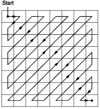
Zig-Zag Sequencing

After quantization, the 2-D matrix is rearranged into a 1-D array. The elements are read in a fashion that gives the coefficients with high energy density first. The sequencing is done in a zig-zag method such that coefficients are arranged in an increasing spacial frequency order. Using this method, the more important coefficients appear earlier on in the series, while the less important ones appear later on. As the high-frequency components are the most likley to round to zero, one will typically end up with a run of zeros at the end of the $64$-entry vector. As the $1 \times 64$ vector contains a lot of zeros, it is more efficient to save the non-zero values and then count the number of zeros between these non-zero values.

Let’s imagine we have this quantized matrix: 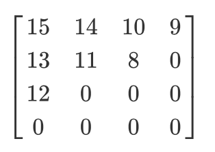The output of zig-zag encoding will be this: $[15,14,13,12,11,10,9,8,0, ... ,0]$. This encoding is preferred because most of the low frequency (most significant) information is stored at the beginning of the matrix after quantization and the zig-zag encoding stores all of that at the beginning of the 1D matrix. This is useful for the compression step that we will not do here.

Exercice [PY-1]

Apply the 4 steps of the JPEG method so as to compress the lena image. Draw the result and save the "zigzag" sequences.

Singular Value Decomposition and Image Compression

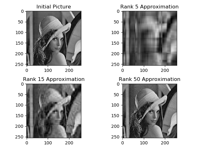To compress the lena image, we apply in this Section the "famous" Theorem called Singular Value Decomposition of a matrix. We will see that the compression of the image is obtained by creating an approximation matrix ${\bf A}_k$ with a lower rank than matrix ${\bf A}$.

The eigenvalue decomposition of a square matrix ${\bf A}={\bf V\Lambda V}^{-1}$ is of great importance and widely used. However, for an $m\times n$ non-square matrix ${\bf A}$, no eigenvalues and eigenvector exist. In this case, we can still find its singular values and the corresponding left and right singular vectors, and then carry out singular value decomposition (SVD). The SVD has many applications, two of which are considered below: image compression and pseudo-inverse calculation of any matrix.

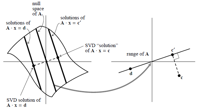
A singular matrix ${\bf A}$ maps a vector space into one of lower dimensionality, here a plane into a line, called the “range” of ${\bf A}$. The “nullspace” of ${\bf A}$ is mapped to zero. The solutions of ${\bf A}{\bf x} = {\bf d}$ consist of any one particular solution plus any vector in the nullspace, here forming a line parallel to the nullspace. Singular value decomposition (SVD) selects the particular solution closest to zero, as shown. The point ${\bf c}$ lies outside of the range of ${\bf A}$, so ${\bf A}{\bf x}= {\bf c}$ has no solution. SVD finds the least-squares best compromise solution, namely a solution of ${\bf A}{\bf x} = {\bf c'}$, as shown.

If $m \gt n$ we obtain by applying the previous result: $$ {\bf A}=\left( \begin{array}[c]{ccc} 2 & 3 & 2\\ 4 & 1 & 0\\ 2 & 2 & 1\\ 4 & 0 & 4\\ \end{array} \right) = {\bf U}{\bf \Sigma}{\bf V}^T $$ where $$ {\bf U}=\left( \begin{array}[c]{cccc} -0.46 & -0.52 & 0.52 & -0.49\\ -0.45 & -0.24 & -0.83 & -0.21\\ -0.36 & -0.39 & 0.09 & 0.84\\ -0.67 & 0.72 & 0.15 & 0.04\\ \end{array} \right) \;\;\;\; {\bf V}^T=\left( \begin{array}[c]{ccc} -0.79 & -0.33 & -0.51\\ 0.04 & -0.87 & 0.49\\ -0.61 & 0.37 & 0.7 \\ \end{array} \right) $$ and $$ {\bf \Sigma}=\left( \begin{array}[c]{ccc} 7.75 & 0.0 & 0.0\\ 0.0 & 2.96 & 0.0\\ 0.0 & 0.0 & 2.48\\ 0.0 & 0.0 & 0.0\\ \end{array} \right) $$ Consequently, the singular values of ${\bf A}$ are $\sigma_1 = 7.75$, $\sigma_2 = 2.96$ and $\sigma_3 = 2.48$

If $m \lt n$ we have for example: $$ {\bf A}=\left( \begin{array}[c]{ccc} 0 & 1 & 1 & 0\\ 2 & 4 & 3 & 4\\ \end{array} \right) = {\bf U}{\bf \Sigma}{\bf V}^T $$ where $$ {\bf U}=\left( \begin{array}[c]{cccc} -0.16 & 0.99\\ -0.99 & -0.16\\ \end{array} \right) \;\;\;\; {\bf V}^T=\left( \begin{array}[c]{ccc} -0.29 & -0.6 & -0.46 & -0.58\\ -0.33 & 0.38 & 0.55 & -0.66\\ -0.3 & -0.64 & 0.64 & 0.31\\ -0.84 & 0.29 & -0.29 & 0.35\\ \end{array} \right) $$ and $$ {\bf \Sigma}=\left( \begin{array}[c]{ccc} 6.79 & 0.0 & 0.0 & 0.0\\ 0.0 & 0.94 & 0.0 & 0.0\\ \end{array} \right) $$ Consequently, the singular values of ${\bf A}$ are $\sigma_1 = 6.79$ and $\sigma_2 = 0.94$

Note that the matrix can be rewritten as a sum of outer products of columns of ${\bf U}$ and rows of ${\bf V}^T$, with the “weighting factors” being the singular values $$ {\bf A} = \sum_{i=1}^{n} \sigma_i {\bf U_i}.{\bf V_i}^T $$ where ${\bf U_i}$ (resp. ${\bf V_i}$) are the column vectors of ${\bf U}$ (resp. ${\bf V}$). If you ever encounter a situation where most of the singular values of matrix ${\bf A}$ are very small (see Exercice [M-1] below), then ${\bf A}$ will be well-approximated by only a few terms. This means that you have to store only a few columns of ${\bf U}$ and ${\bf V}$ and you will be able to recover, with good accuracy, the whole matrix. If your matrix is approximated by a small number $k$ of singular values, then this computation of $A.x$ takes only about $k(m + n)$ multiplications, instead of $mn$ for the full matrix.

Exercice [M-1]

Let ${\bf A} \in {\mathcal M}_{m,n}({\mathbb R})$ be a matrix of rank $r \leq \min{(m,n)}$. In the following we consider the Frobenius norm or the $2$-norm matrix. We want to approximate or find the closest matrix ${\bf A_k}$ of rank $k \lt r$ to matrix ${\bf A}$. Observe firstly that this best approximation problem makes sense since we have defined a distance (via a matrix norm) on ${\mathcal M}_{m,n}({\mathbb R})$. However, even if the existence of best approximants does not offer any difficulty (remember that the matrix norm is a continuous function), the question of uniqueness as well as that of an explicit form of best approximants remain posed.

• Show that $$ \min_{\rank({\bf X}) \leq k} \left\| {\bf A}-{\bf X} \right\| _{F} \;\;\text{and} \;\;\min_{\rank({\bf X}) \leq k} \left\| {\bf A}-{\bf X} \right\| _{2} $$ have the same solution $ {\bf A}_k = \sum_{i=1}^{k} \sigma_i {\bf U_i}.{\bf V_i}^T $ where ${\bf U_i}$ (resp. ${\bf V_i}$) are the column vectors of ${\bf U}$ (resp. ${\bf V}$).

• Show that for any $0 \lt k \lt r$, $ \left\| {\bf A}-{\bf A}_k \right\| _{F} = \sqrt{\displaystyle{\sum_{i=k+1}^{r}\sigma_i}} $ and $ \left\| {\bf A}-{\bf A}_k \right\| _{2} = \sigma_{k+1} $

Exercice [PY-2]

We use scipy.linalg to obtain the SVD of ${\bf A}$. It yields [U,S,Vh] = sl.svd(A) (this algorithm uses the QR-decomposition) (we recall that Vh=$V^*$ and $S$ is a vector). If we only want the singular values in a vector $s = (\sigma_1, . . . , \sigma_n)$ we have to use
s = sl.svdvals(A)

1. Create a random matrix $A$ of size 30 × 50 such that each coefficient follows a random law: $a_{i,j} \in U[−5, 5]$ (see random.rand or uniform).
2. Draw the relation between the singular values of $A$ and the spectrum of $A^TA$ and $AA^T$ (sort the values by using sorted).
3. Create matrix $B$ being the best least squares approximation of rank $k$ of $A$. Calculate the error of this approximation with the $2$-norm and the Schur (Frobenius) norm for $0 \lt k \lt r$ with $(r = rg(A))$ and the draw the error curves. Compare these errors (you can use the results of the exercice above)
4. Use the command data = mpimg.imread(’lena.png’) so as to associate the pixel values of the image to the data matrix of size (256 × 256)
5. Viewing the photo can be done with the plt.imshow (data, cmap = "gray") command. You can add a threshold for the gray values, by adding the parameters vmin = 0 and vmax = 255.
6. Calculate the singular value decomposition of $A$ then display the minimum and maximum of coefficients of ${\bf A}$, ${\bf U}$, ${\bf V}$ as well as the singular values ​​$ \sigma_1 $ and $ \sigma_n $.
7. The plt.subplots command will allow you to create subplots:
   fig, ax = plt.subplots (2,2, figsize = (10,10))
   Display on 4 graphics side by side the image of Lena as well as the approximations of rank 5, 15 and 50 of this same image. Add titles to each subplot. How much memory space saved with the last rebuild?

References

- C. Eckart, G. Young, The approximation of one matrix by another of lower rank. Psychometrika, Volume 1, 1936, Pages 211–8. doi:10.1007/BF02288367
- W. B. Pennebaker and J. L. Mitchell, Van Nostrand Reinhold, JPEG still image data compression standard, New York, 1992
- Golub, G.H., and Van Loan, C.F. 1989, Matrix Computations, 2nd ed. (Baltimore: Johns Hopkins University Press), x8.3 and Chapter 12.
- H.J. Nussbaumer (1981) Fast Fourier Transform and Convolution Algorithms. Springer-Verlag.
- Forsythe, G.E., Malcolm, M.A., and Moler, C.B. 1977, Computer Methods for Mathematical Computations (Englewood Cliffs, NJ: Prentice-Hall), Chapter 9