Control Engineering Application

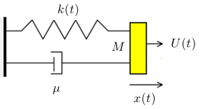
Spring mass control

In this exercice we want to calculate the control $U(t)$ such that the mass follows a given trajectory $x_{ref}(t)$. \[ \left\{ \begin{array}{l} Mx''(t)+\mu x'(t) +k_1 x(t) + k_2 (x(t))^3 = U(t) \\ x(0) = 0 \\ x'(0)= 1\\ \end{array}\right. \]

• Bang Bang control
• PID control

The "Bang Bang" control implementation

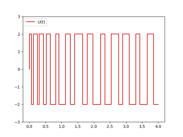
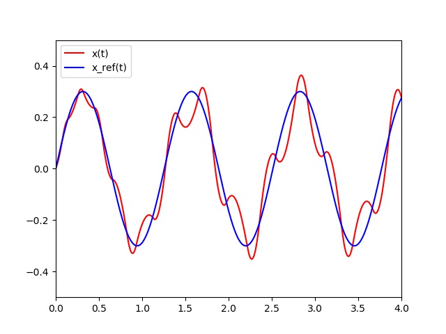
A bang–bang controller is a feedback controller that switches abruptly between two states. The control value $U(t)$ can only take two values: $U_{max}$ or $-U_{max}$ respectively. This value only depends on the sign of the error between the reference value $x_{ref}(t)$ and the current state $x(t)$ at time $t$. In the following Figure, we can see the current state $x$ of the mass and the $x_{ref}$ functions at each time $t$.

$K_p$ being proportionality coefficient of the error to be set manually. In practice, the control values are bounded. Consequently, we assume that $U = \min(K_p*error,U_{max})$ or $U = \max(K_p*error,-U_{max})$ if $error < 0$.

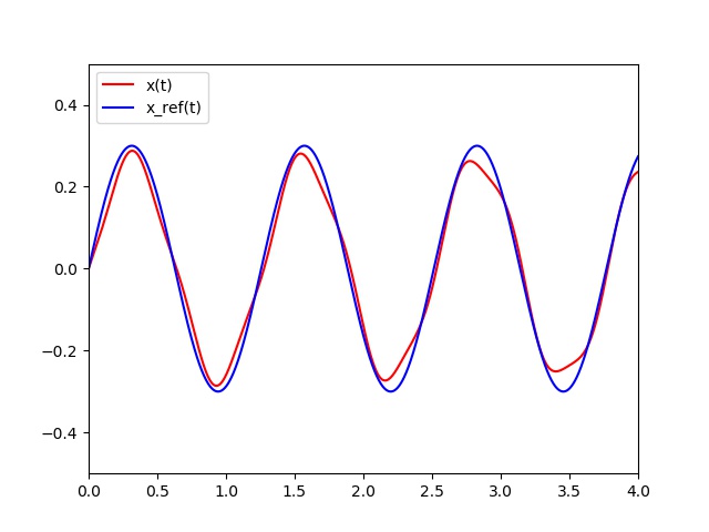
To follow the reference, we apply the proportional regulator control strategy. At each sampling control period, here $10ms$, we calculate the error = x_ref(t) - x_state(t) and we apply the previous control strategy. As we can see, control $U$ has small steps according to the control period. In fact, we assume the control applied during a sampling period is constant.

        Every x milliseconds, do:
        
            error = x_ref - x_measure
            sum_errors += error
            variation_error = error - previous_error
            U = Kp * error + Ki * sum_errors + Kd * variation_error
            previous_error = error
        

The adjustment of the coefficients $K_p$, $K_i$ and $K_d$ of a PID can be done "by hand" by trial and error. First of all, know that it is useless to want to adjust the three coefficients at the same time! There are too many possible combinations and finding a successful triplet would be a feat. It is better to go there in stages. First of all, it is necessary to set up a simple proportional regulator (the coefficients $K_i$ and $K_d$ are therefore zero). By trial and error, it is necessary to adjust the coefficient $K_p$ in order to improve the response time of the system. That is to say, you have to find a $K_p$ that allows the system to approach the setpoint very quickly while being careful to keep the system stable: the system must not respond very quickly while oscillating many ! Once this coefficient has been set, we can move on to the coefficient $K_i$. This will make it possible to cancel the final error of the system so that it respects exactly the instruction. It is therefore necessary to adjust $K_i$ to have an exact response in a short time while trying to minimize the oscillations provided by the integrator! Finally, we can go to the last coefficient $K_d$ which makes the system more stable. Its adjustment therefore makes it possible to reduce the oscillations.

The perfect PID does not exist, it is all a question of compromise. Some applications will allow an overshoot to improve the stabilization time, while others will not allow it. Everything therefore depends on the specifications. Each of the coefficients has a role to play on the response to a setpoint: Static error is the final error once the system is stable. This error must be null. To decrease the static error, it is necessary to increase $K_p$ and $K_i$. The overshoot is the ratio between the first peak and the setpoint. This overshoot decreases if $K_p$ or $K_i$ decrease or if $K_d$ increases. The rise time corresponds to the time it takes to reach or exceed the setpoint. The rise time decreases if $K_p$ or $K_i$ increase or if $K_d$ decreases. The stabilization time is the time it takes for the signal to make an error of less than 5% of the setpoint. This stabilization time decreases when $K_p$ and $K_i$ increase. To give you a little idea of ​​the value of the coefficients during your first tests, you can look at the side of the Ziegler – Nichols method. This method makes it possible to determine $K_p$, $K_i$ and $K_d$ according to your specifications. Coefficients $K_i$ and $K_d$ depend on the sampling frequency of the system. Indeed, the integrator will add up the errors over time! If we sample twice as fast, we will add twice as many samples. Suddenly, the coefficient $K_i$ will have to be divided by $2$. Conversely, for the derivative, if we double the sampling frequency, it will be necessary to double the coefficient $K_d$ in order to keep the same performances of the PID. The higher the sampling frequency, the better the PID will be. Indeed, the more often we sample the more precise the integration and derivative will be.

• By assuming that $M = 0.1$, $\mu= 0.1$, $k_1 = 5$ and $k_2 = 1$, define the following python vector function which modelize this second order system:

                  def F(t,V,U):
                      #To Do
                      return  
              

Python Solution

            M = 0.1
            mu= 0.1
            k1 = 5
            k2 = 1

            def F(t, V, U):
                L=[V[1],U/M-mu/M*V[1]-k1*V[0]/M-k2/M*V[0]**3]
            return L
        

• We would like to find the value $U$ of the force that we have to apply at each 0.01s so as to follow a reference value of $x$ denoted by $x_{ref}(t)$.
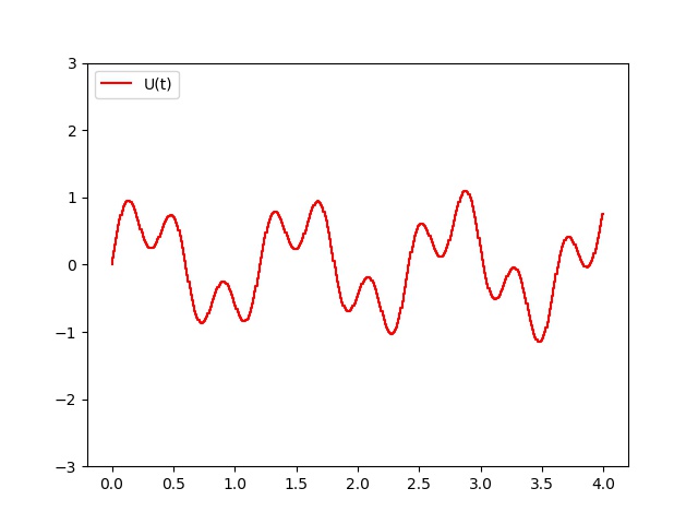
  We assume that $$x_{ref}(t) = A sin(5t) \quad \text{for} \quad t \in [0,10], \quad \text{with} \quad A=0.3$$ We set that $U(t)$ can only take two values according the sign of the error between the reference value and the current state $x$: $U_{max}$ or $-U_{max}$ respectively where $U_ {max}=2N$. This a "bang-bang" type control. By using the Runge-Kutta of order $2$ at each step, define the control $U$ to be applied at each $0,01s$ so that the mass can be able to follow the reference $x_{ref}(t)$.

Python Solution

        A = 0.3
        def x_ref(t):
            return A*np.sin(5*t)

        def BangBang(V0,T,dt,pas,Umax):
            h=dt/pas
            nb = int(T / h)+1
            t=0
            X=[0]
            Y=[V0[0]]
            V1=V0
            BB=[]
            t_u = []
            for i in range(nb):
                
                if i % pas == 0:
                    err = x_ref(t)-V1[0]
                    U = err
                    if U>0:
                        U = Umax
                    elif U < 0:
                        U = -Umax
                    else:
                        U = 0.0
                        
                    BB.append(U)
                    t_u.append(t)
                
                k1=np.dot(h,F(t,V1,U))
                k2=np.dot(h,F(t+h,V1+k1,U))
                V2=V1+(k1+k2)/2.0
                t=t+h
                Y.append(V2[0])
                X.append(t)
                V1=V2
                
            return X,Y,t_u,BB

        V0 = [0,1]
        T = 4
        dt = 0.01
        pas = 100
        Umax = 2
        Kp = 20
        
        # Bang Bang strategy
        t,X,t_u,U = BangBang(V0,T,dt,pas,Umax)
        plt.xlim(0,T)
        plt.ylim(-0.5,0.5)
        pX = plt.plot(t,X,'r', label="x(t)")
        s = np.linspace(0,T,int(1/dt)*pas)
        xref = x_ref(s)
        px = plt.plot(s,xref,'b', label="x_ref(t)")
        plt.legend(loc='upper left')
        plt.savefig('BRessortX.jpg')
        plt.clf()
        plt.ylim(-3.,3.)
        pU = plt.step(t_u,U,'r', label="U(t)")
        plt.legend(loc='upper left')
        plt.savefig('BRessortU.jpg')
        plt.clf()
        

• Apply the proportional regulator strategy and find the best $K_p$ value.

  Python Solution

          def PC(V0,T,dt,pas,Umax,Kp):
              h=dt/pas
              nb = int(T / h)+1
              t=0
              X=[0]
              Y=[V0[0]]
              V1=V0
              PID=[]
              t_u = []
              for i in range(nb):
                  
                  if i % pas == 0:
                      err = x_ref(t)-V1[0]
                      U = Kp*err
                      if U>Umax:
                          U = Umax
                      if U <-Umax:
                          U = -Umax
                          
                      PID.append(U)
                      t_u.append(t)
                  
                  k1=np.dot(h,F(t,V1,U))
                  k2=np.dot(h,F(t+h,V1+k1,U))
                  V2=V1+(k1+k2)/2.0
                  t=t+h
                  Y.append(V2[0])
                  X.append(t)
                  V1=V2
                  
              return X,Y,t_u,PID
  
          V0 = [0,1]
          T = 4
          dt = 0.01
          pas = 100
          Umax = 2
          Kp = 20
  
          # Proportional strategy
          t,X,t_u,U = PC(V0,T,dt,pas,Umax,Kp)
          plt.xlim(0,T)
          plt.ylim(-0.5,0.5)
          pX = plt.plot(t,X,'r', label="x(t)")
          s = np.linspace(0,T,int(1/dt)*pas)
          xref = x_ref(s)
          px = plt.plot(s,xref,'b', label="x_ref(t)")
          plt.legend(loc='upper left')
          plt.savefig('PRessortX.jpg')
          plt.clf()
          plt.ylim(-3.,3.)
          pU = plt.step(t_u,U,'r', label="U(t)")
          plt.legend(loc='upper left')
          plt.savefig('PRessortU.jpg')
          

• Do the same for the the integral proportional regulator (PI), The proportional derivative regulator (PD) and the derivative integral proportional regulator (PID). What is the optimal strategy according to which criteria?

• Draw for each control type the $U$ and the $x$ solutions for these strategies.

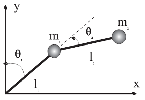
Control of a two axis robot

In this exercice we want to calculate the two controls that we have to apply to a two axis robot so as to follow a given trajectory.

• By assuming that $m_1 = 40kg$, $l_1 = 0.85m$, $g = 9.81$, $m_2 = 125kg$ and $l_2 = 0.5m$ then define the following python vector function which modelize this robot system:

                      def F(t,V,U):
                          #To Do
                          return  
                  

Hint of Solution
To solve this problem we set :\[ V(t) =\left(\begin{array}{c} \theta_1(t) \\ \overset{.}{\theta}_1(t) \\ \theta_2(t) \\ \overset{.}{\theta}_2(t)\end{array}\right).\] By using the previous differential equations, you can obtain the $F$ function where $U$ is now a list of two values: the two axis torques $U_1$ and $U_2$.
• By using a Runge-Kutta of order 4 algorithm apply the Bang Bang control strategy for each torques $U_1$ and $U_2$ so as to follow the reference angular functions: \[ \theta_1^*(t) := \dfrac{\pi}{4} sin(t) \] \[ \theta_2^*(t) := \dfrac{\pi}{4} cos(t) \] We choose $0.01s$ for the value of the control sampling.
• Do the same for a PI control strategy.
• Draw $U_1$, $U_2$, $\theta_1$ and $\theta_2$.

References

- J.H. Ahlberg, E.N. Nilson & J.L. Walsh (1967) The Theory of Splines and Their Applications. Academic Press, New York.
- C. de Boor (1978) A Practical Guide to Splines. Springer-Verlag.
- G.D. Knott (2000) Interpolating Cubic Splines. Birkhäuser.
- H.J. Nussbaumer (1981) Fast Fourier Transform and Convolution Algorithms. Springer-Verlag.
- H. Späth (1995) One Dimensional Spline Interpolation. AK Peters.